Forced isotropic turbulence on JHTDB

Problem

Turbulence theory, once written out, makes specific and testable claims about any flow that satisfies its assumptions. The AER1324 course project at UTIAS was an excuse to take those claims and push them against a real dataset — to see which pieces actually land, and from which angle.

Approach

The data source was the Johns Hopkins Turbulence Database forced-isotropic-turbulence DNS: a periodic cubic domain at $1024^3$ resolution, $Re_\lambda \approx 433$, energy continuously injected at low wavenumbers to hold the flow in a statistically steady state. Sampling the field through the JHTDB API, I put together a workflow that went from DNS access to statistical analysis to spectral analysis to structure identification in one line, and could be rerun on a different slice without refactoring.

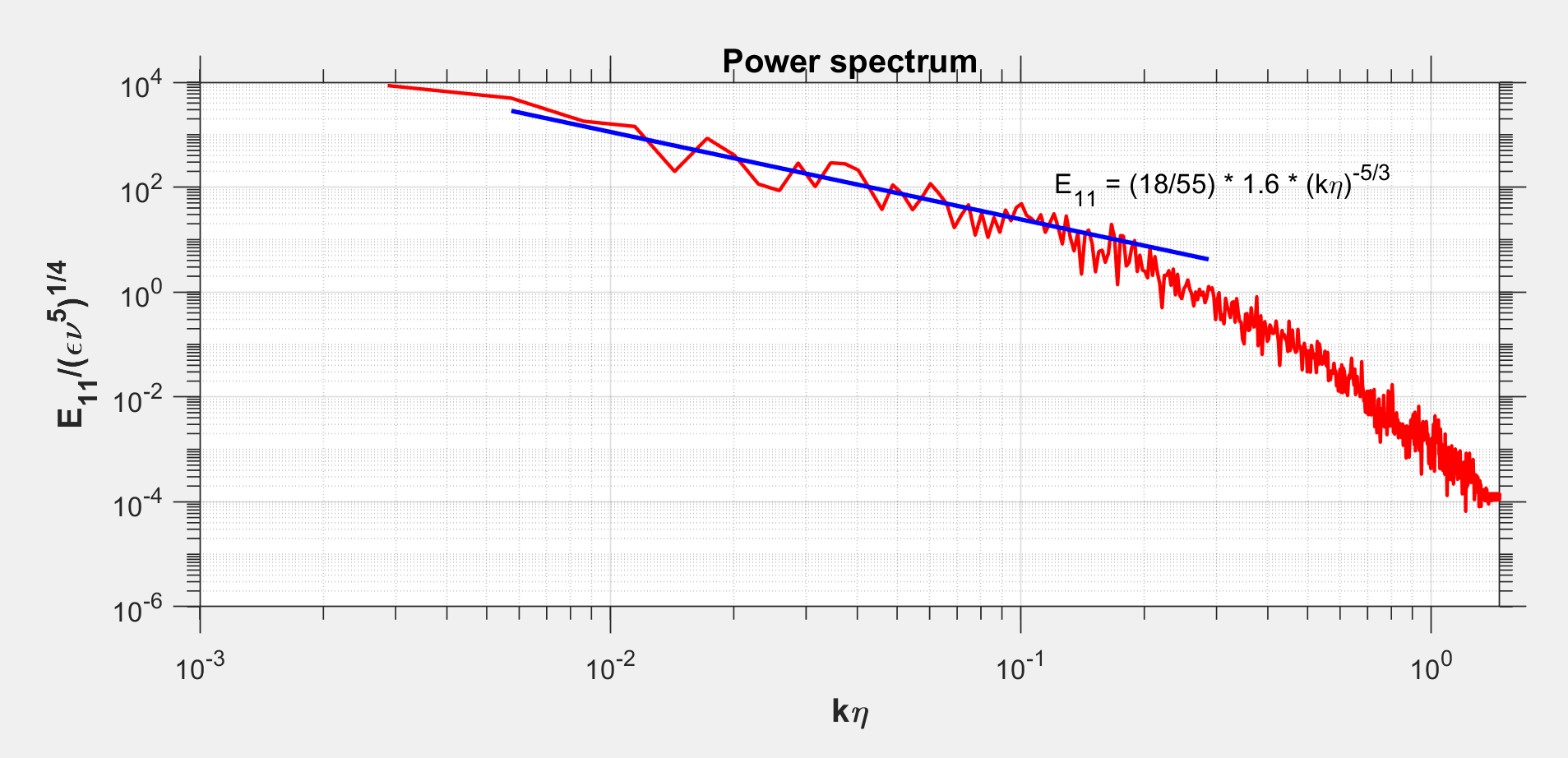
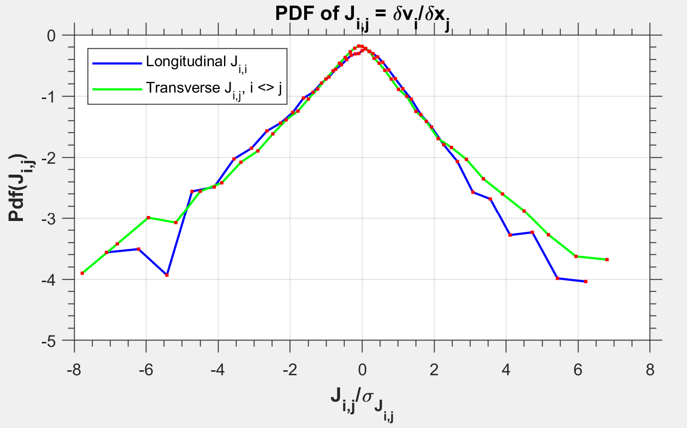
Two lenses ran through everything. Statistical: velocity and pressure PDFs over the full domain versus over a $1/64$ subdomain, plus strain-rate statistics, as a test of Gaussianity at large scales and intermittency at small ones. Spectral: 1D power spectra $E_{11}(k)$ averaged over randomly oriented lines, compared against Kolmogorov’s $k^{-5/3}$ and used alongside DNS gradients to estimate $\varepsilon$ and the Kolmogorov scale $\eta$.

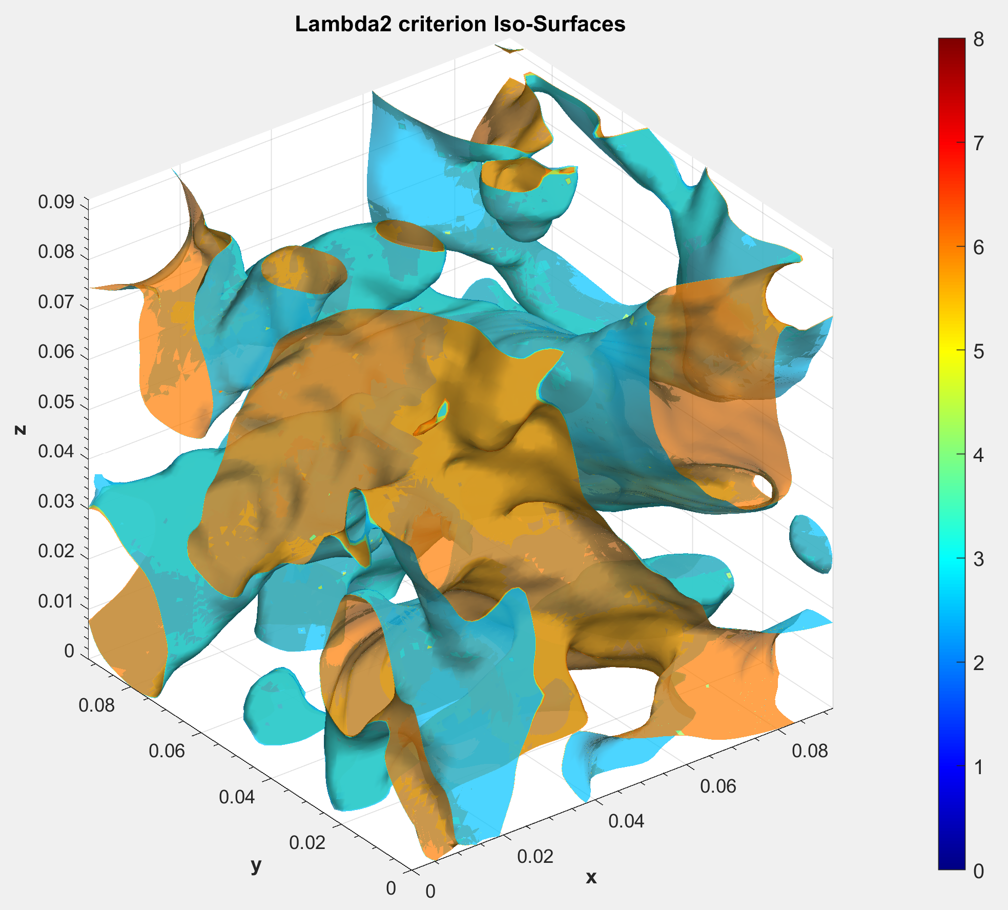
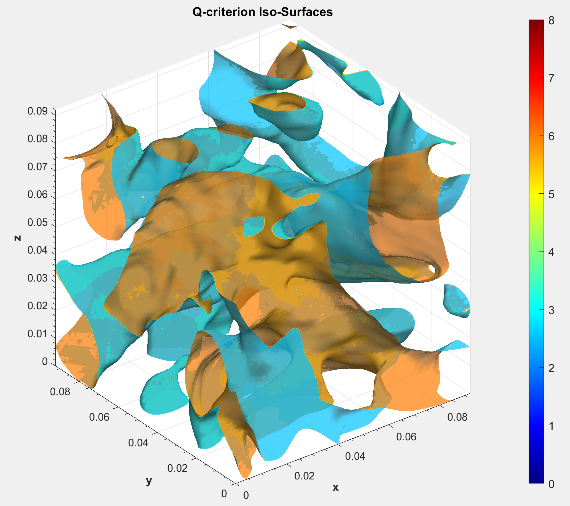
Structure identification used Q and $\Lambda_2$ on the focused region, with the pressure Hessian and the complex eigenvalues of the velocity gradient as supporting diagnostics. Q picks up the diffuse vortical background; $\Lambda_2$ filters down to compact cores. The pair reveals more than either alone.

Result

The statistics behaved as isotropic turbulence is supposed to. Full-domain velocity and pressure PDFs were close to Gaussian; focused-region PDFs picked up the classical heavier tails and sharper peaks of intermittency. The compensated spectrum showed a clean $k^{-5/3}$ region in the inertial range and the steeper drop of the dissipation range beyond it. The DNS-estimated $\eta$ confirmed the grid resolves the smallest scales.

The geometric story lined up. Q iso-surfaces covered a broad vortical background; $\Lambda_2$ resolved the compact cores, and the pressure Hessian traced their footprint in the curvature of the pressure field. Different mathematical views of the same flow agreed on where energy is concentrated and dissipated.

What I’d do differently

I would frame more of the workflow as a reusable JHTDB toolkit from the beginning. Much of what the project produced is now sitting in one project-specific notebook; broken into small utilities — field sampling, line spectra, Q/$\Lambda_2$ — the same code would carry into a wall-bounded or anisotropic dataset without rework.