Why this codebase
The Lomax–Pulliam–Zingg two-book CFD curriculum sets the theory and the algorithms in one consistent voice: Book 1 is the analytical spine — operator analysis, modified wavenumbers, stability regions, modified-PDE character — and Book 2 is the algorithmic spine, three structurally different solver families on the same governing equations. Reading the books is one thing; building the codebase that runs every result they describe is the thing that makes the theory operational.
CFDLab is that codebase — mine, written from scratch in Python, still developing.
What it is
Three full from-scratch quasi-1-D Euler solvers, one analytical-probe layer, one shared kernels module, and a 74-entry worked Exercise Guide. Forty-three numerical baselines pinned by per-project MD5 hashes and CI-enforced on every push.
The reading order on this page mirrors the codebase. Analytical foundations first — the modified wavenumber, the TVD region, modal decay rates that everything else has to obey. Then the three solver projects, each on the canonical problem it was built to handle. The cross-project JST-vs-Roe shock-tube comparison closes the page; with the groundwork in place, the contact-discontinuity result reads as an outcome rather than a fact.
Analytical foundations
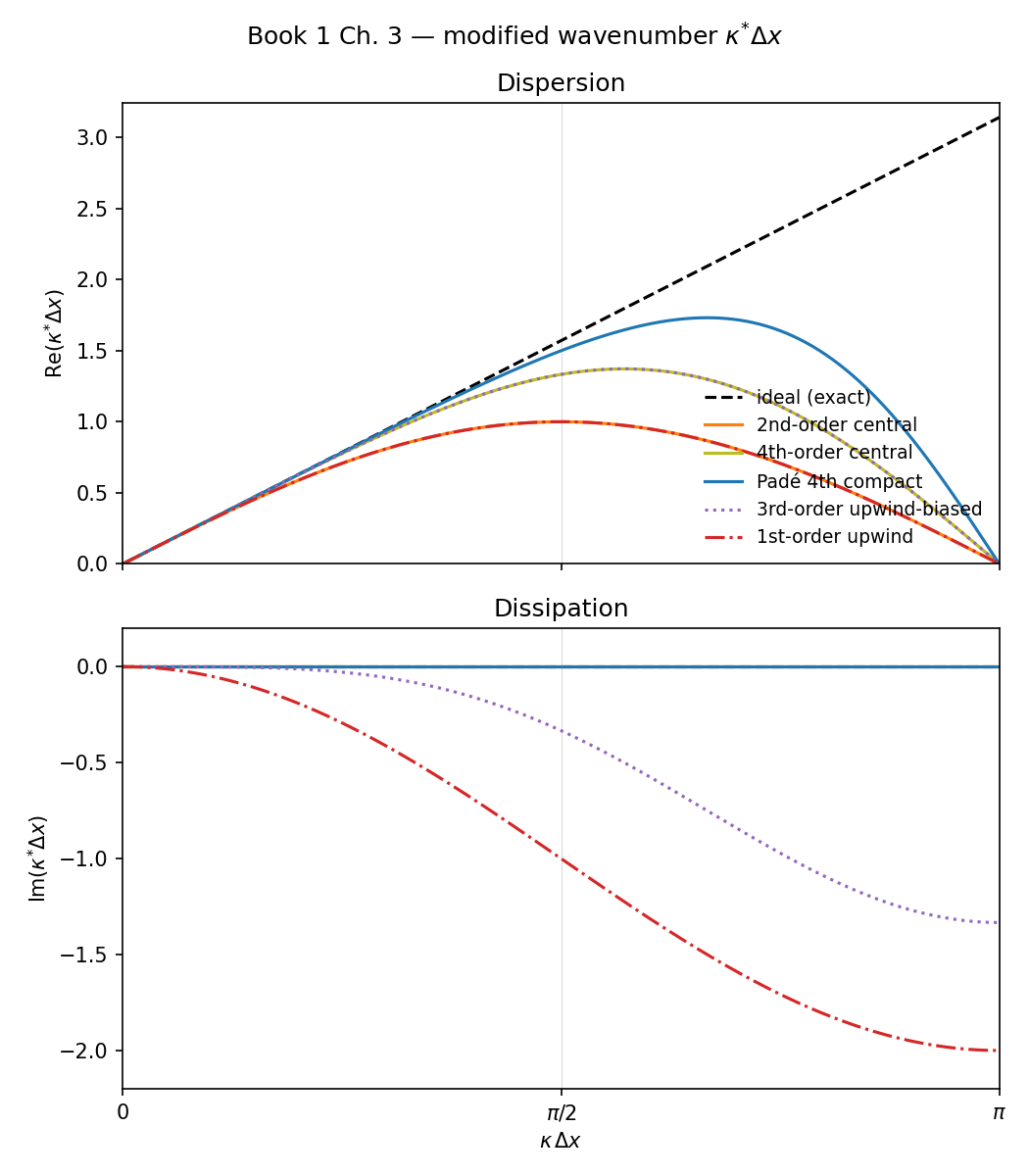
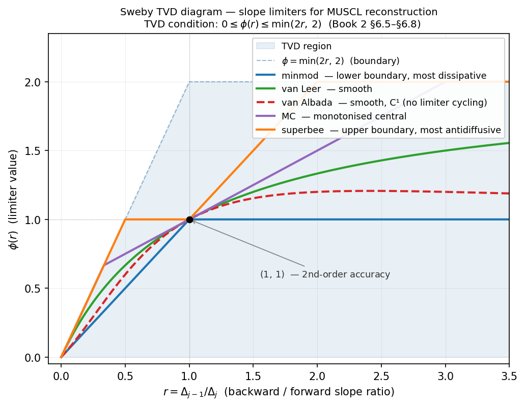
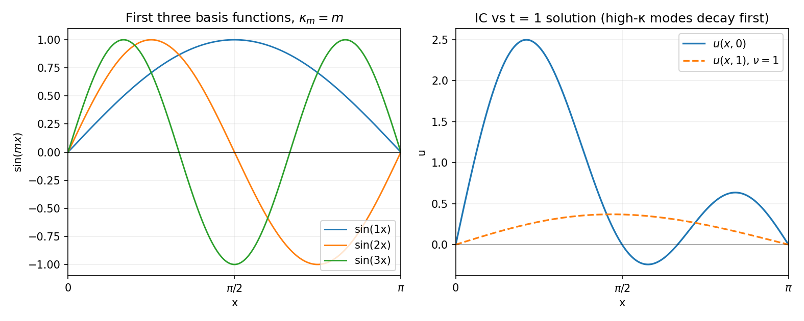
Three figures, all from the analytical-probe layer. The modified wavenumber sets the reading frame: every scheme below the line is a choice in phase and amplitude error per resolved wave. The Sweby diagram is the bridge from pure FD analysis to shock-capturing — limiters live inside that region or they are not TVD. The diffusion modal decay closes the lead trio with the time-domain side of the same machinery: discrete decay rates against the analytical reference, mode by mode.
These are not anchored to any one solver. They are the language the solvers below speak.
Three solver projects
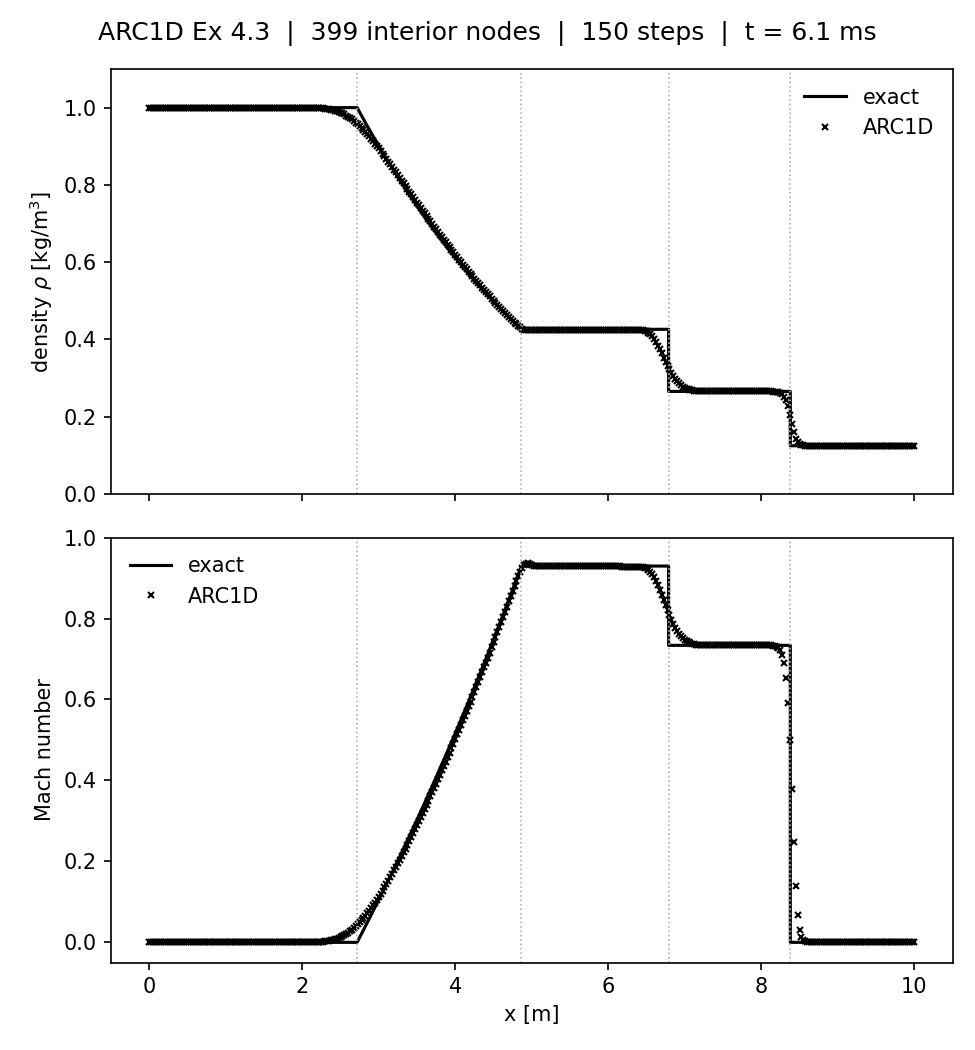
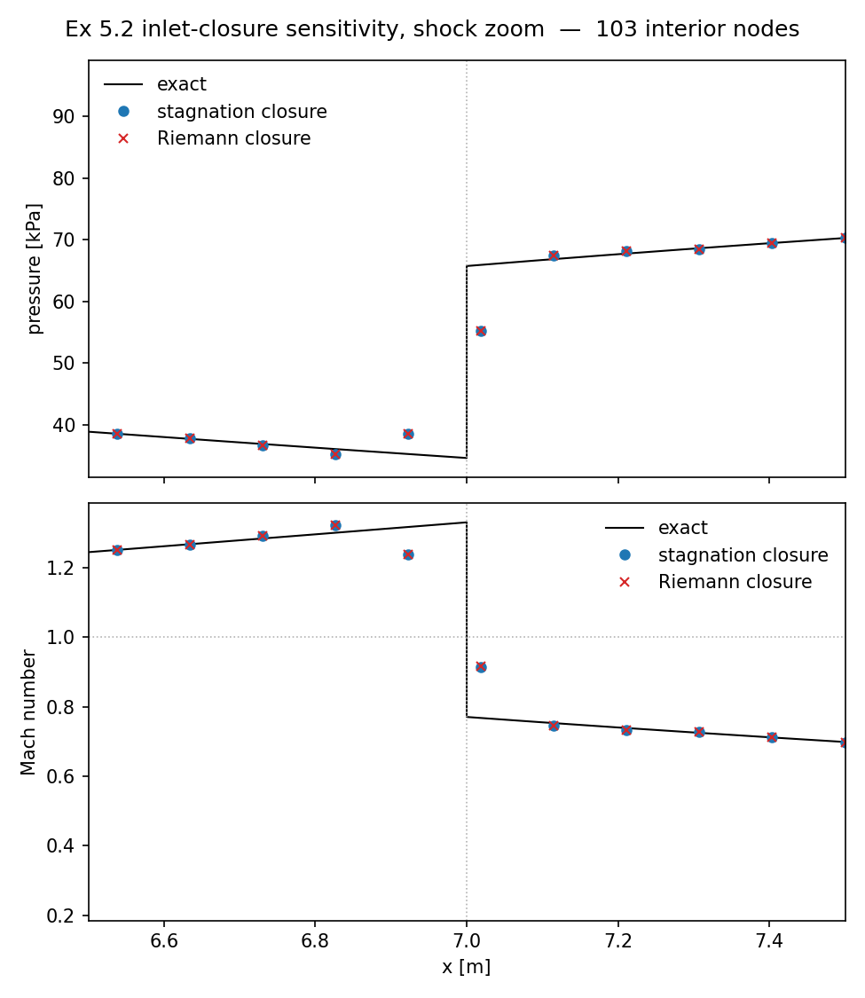
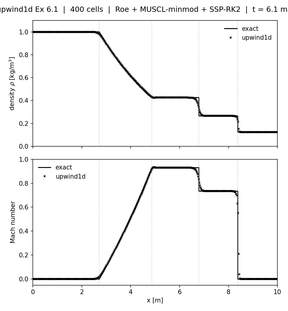
The three Book 2 solvers are structurally different. ARC1D is the Ch.4 lane — implicit finite difference with JST scalar artificial dissipation in delta-form, solved by block-Thomas. FLOMG is Ch.5 — explicit finite volume with five-stage Van der Houwen Runge–Kutta time-marching wrapped in a FAS multigrid driver. upwind1d is Ch.6 — Roe approximate Riemann + MUSCL piecewise-linear reconstruction + TVD slope limiting + SSP-RK2.
Each runs on the canonical problem the project was built to handle. ARC1D does Sod and the transonic nozzle; FLOMG does steady transonic with multigrid; upwind1d does Sod with shock-capturing. The figures here are per-solver — each solver, on its own, doing its own work.
A note on FLOMG: the explicit-FV multigrid lane is purpose-built for steady flows with a single shock, not for the Sod shock-tube transient. Showing FLOMG on transonic rather than on Sod is the honest figure for that lane.
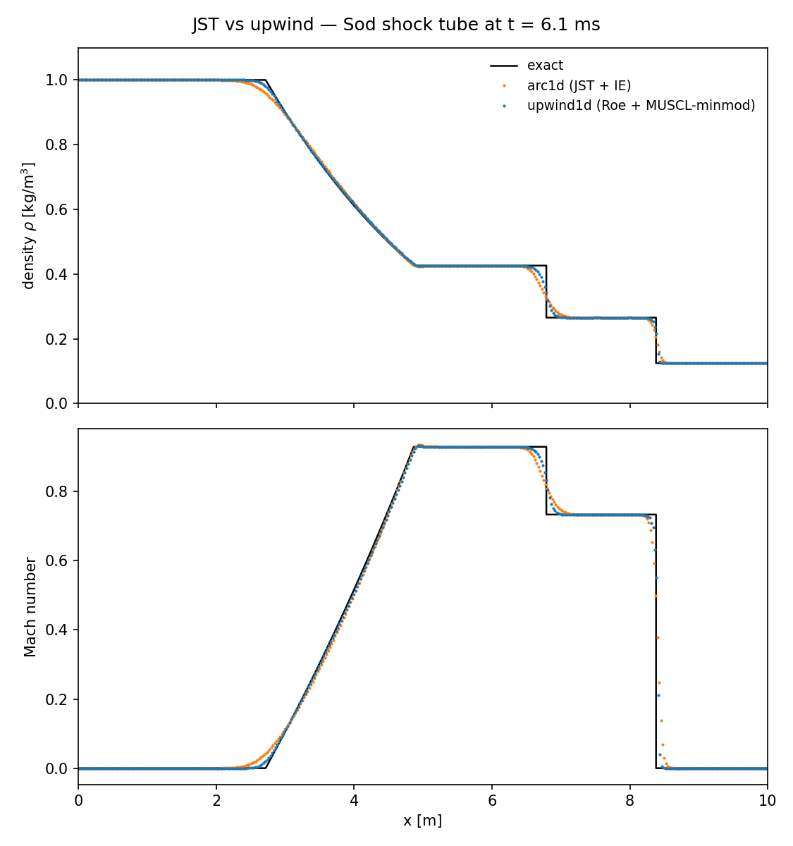
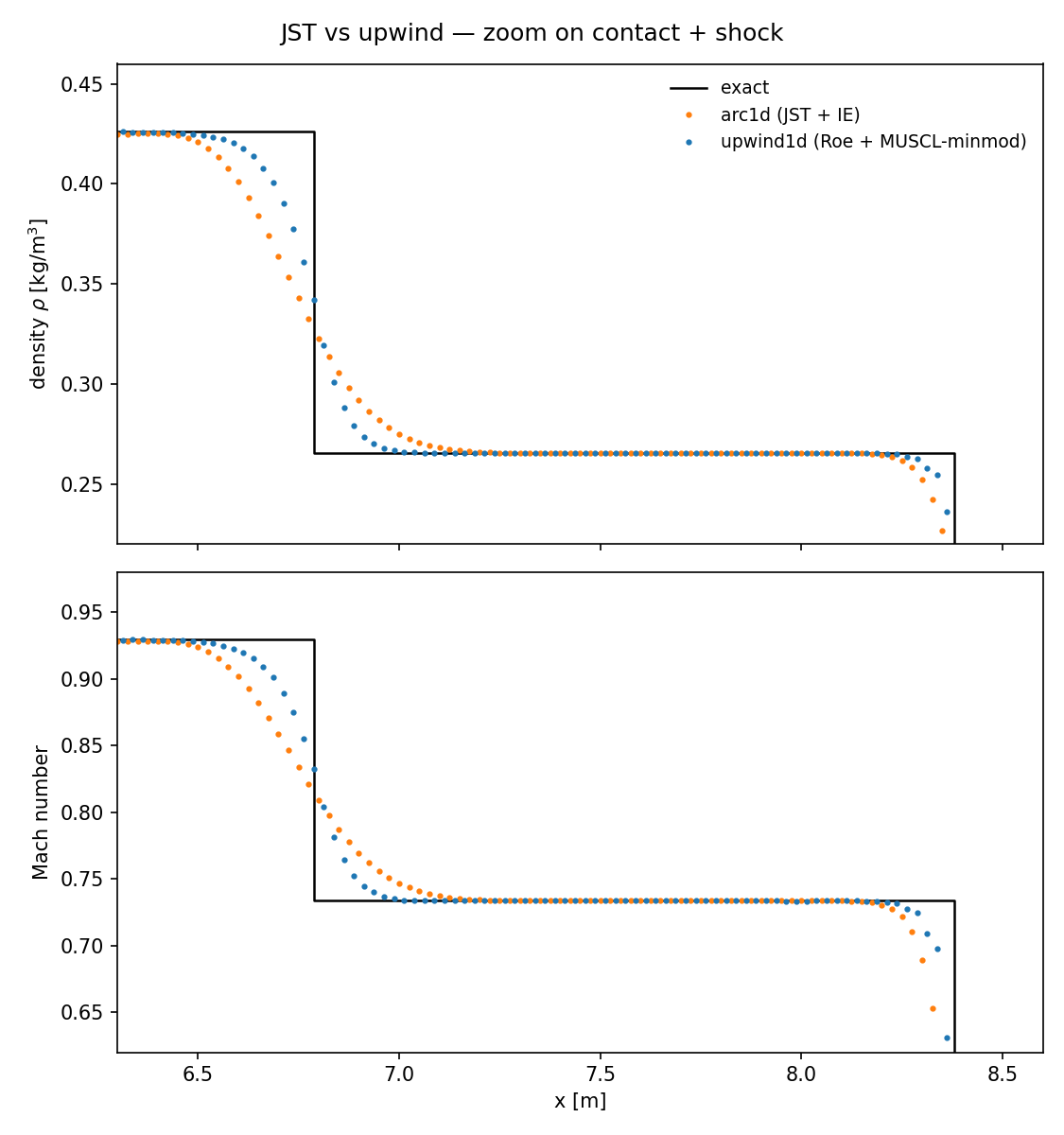
Cross-project shock-tube comparison
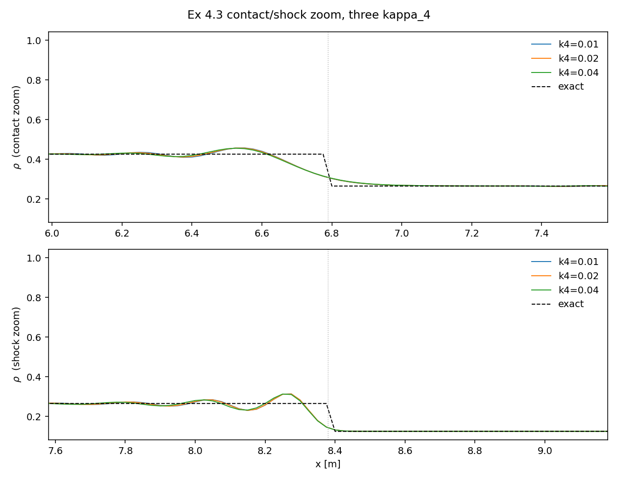
The payoff. With the analytical frame and the three solver lanes on the screen, the JST-vs-Roe Sod overlay reads correctly: the rarefaction → contact → shock structure across the whole domain (full overlay), then the contact zoom that makes Book 2’s central algorithmic argument visible in one image. The scalar-pressure-sensor JST artificial dissipation smears the contact discontinuity over about three cells; characteristic-decomposition Roe + MUSCL upwinding holds it in about one. That is the result the rest of the page exists to support.
What it earns
CFDLab’s payoff is not “I have a solver.” It is I can read a method-property probe before I run a case and know what the case will say. The discipline of building three structurally different solvers against the same governing equations, with the analytical layer right there to consult, is the discipline that lets a workflow elsewhere — an OpenFOAM run on the cluster, a high-order SBP scheme on a model PDE — give up its pathologies before the dashboard hides them.
The plateau is v0.6-two-book-exercise-guide. The next development lanes are recorded; the next phase is whichever one earns its way in next.
Analytical foundations
Three solver projects
Cross-project shock-tube comparison