MEng coursework · UTIAS AER1216 · Group 10 · Fall 2024
One carrier aircraft, five survey drones. Sizing it means solving for a weight that depends on itself.
The course brief is a request from Environment Canada for a wildlife survey flown across northern Canada: one fixed-wing carrier, 930 km unrefuelled, five quadrotors and 60 kg of electronics aboard. To size that aircraft you need its takeoff weight. To know its takeoff weight you need to know what fraction of it is structure, and that fraction depends on the takeoff weight. That circular dependency is what the first nine iterations are for.
What the client asked for
The briefThe brief casts Environment Canada as the client. Sites across northern Canada have been identified as wildlife habitat. They are too far apart and too remote to resupply, so a fixed-wing carrier has to reach all of them and come home on one tank, and it has to release and recover the small multirotors that do the actual surveying. The requirements below are the senior engineer's, quoted from the brief. Every one of them turns into a number the design has to hit.
Two vehicles, then. The carrier is a fixed-wing aircraft that flies the 930 km, carries five surveyors and 60 kg of solar charging electronics, never lands at a site, and is stable enough to fly itself. The surveyor is a quadrotor dropped by parachute that has to hold station within 5 m of a moving animal for a hundred seconds.
Under the project sit three problem sets: thin aerofoil theory on the NACA 0012 and 4412, a propeller blade-element analysis checked against wind-tunnel data, aircraft range and endurance and climb, and a hexarotor performance study using blade element theory with the Coleman inflow model. The project is the subject here; the assignments come in only where the project depends on them.
This was a group project. The report, the design decisions and the conclusions are Group 10's. What is individually attributable is the code: which files were supplied with blanks in them and what went into the blanks. Chapter 07 lays that out file by file.
Gross weight depends on gross weight
SizingHere is the problem that makes conceptual design different from analysis. You want the gross takeoff weight, W0. It is the sum of three things: the payload, which the client fixed at 66.69 kg; the fuel; and the empty structure. Fuel is easy enough as a fraction of gross weight, because the range equation gives you how much of the aircraft you burn per segment. The empty structure is the trap. Bigger aircraft are proportionally lighter in structure, so the empty fraction depends on the answer you are trying to find.
Write both statements of the empty fraction and the trap becomes a picture. Raymer's fit is an empirical curve through decades of real aircraft:
We/W0 = A · W0C, with A = 0.96 and C = −0.05
and the mission demands a second, completely different statement: whatever is left after payload and fuel.
We/W0 = 1 − Wf/W0 − Wpayload/W0
The first falls slowly with size. The second rises steeply, because a fixed 66.69 kg of payload is a smaller and smaller share of a growing aircraft. They cross once. That crossing is the only gross weight at which the aircraft is consistent with itself, and it is the whole of the figure at the top of the page.
Narration
01 A guess that does not matter
The loop starts wherever you tell it to. This is the initial guess written into the earlier revision of the script, 4529.4363 N, about 38 % heavier than the answer. It does not matter which guess it was. The map is a contraction, so every starting point in range walks to the same place, and that is the property that makes a circular definition into a calculation.
02 Walking in
Each pass takes the current weight, asks Raymer's fit what fraction of it would be structure, and asks the mission what gross weight that fraction implies. The answer becomes the next guess, and the error falls by roughly a factor of five a pass, which is what a contraction with a shallow slope looks like. By pass six it is polishing. The empty fraction has settled and the weight is moving in the third decimal. The loop stops when a pass changes the answer by less than a thousandth of a newton, which is a tenth of a gram of aeroplane.
03 Closed
Converged, in nine passes, at 3283.1777 N. That exact value is what the next revision of the script carries as its initial guess, so the two files are provably one calculation written twice, and the number reported here is the number the coursework reported.
Started from the initial guess in the earlier revision of the script, 4529.4363 N, the loop converges in nine passes to 3283.1778 N. new the walk itself: the coursework solved this and never drew it.
The fuel fraction that feeds the closure line is four multiplications. Takeoff costs 3 % of the weight, climb 1.5 %, and the descent and loiter 0.5 %; those come straight off Raymer's table. Cruise is the only one that is computed, and it is the Breguet range equation rearranged: how much of the aircraft you have to burn to fly 1000 km at 100 m/s with a lift-to-drag ratio of 12.25. The product of the four is the fraction of the aircraft still flying at the end of the mission, and 6 % is added back for trapped and reserve fuel.
From a weight to a wing
GeometryA gross weight is not yet an aeroplane. The next step is wing area, and the quantity that sets it is wing loading, the weight carried per square metre. Low wing loading means a big wing: slow, gentle, able to take off short, and draggy. High wing loading means a small wing: fast and efficient in cruise, but it needs a long runway and it stalls fast. Every airframe decision after this one is downstream of that single trade.
The script works the takeoff constraint, Raymer's takeoff parameter against the chosen power loading and the maximum lift coefficient, and gets W/S = 84.92 kg/m2, which for 334.68 kg is a wing of 3.941 m2. The unit is mass over area, not weight over area: in newtons the same loading is 833 N/m2, and the 547 N/m2 reported further down is the same aircraft on the 6 m2 wing it was actually given.
The next line of the script reads S_ref = 6.
That is a design decision, not a derivation, and it is a defensible one: the stall requirement is the binding constraint here, not takeoff, and a bigger wing is how you get under 20 m/s. But the report presents 6 m2 without mentioning that the calculation above it produced 3.94, and every number downstream, span, chord, stall speed, range, comes from the 6. Both numbers stand here and the original is not repaired. why this matters
Aspect ratio 10 was chosen for a long cruise: a long thin wing sheds less energy into its own tip vortices. Span and chord follow from area and aspect ratio and nothing else.
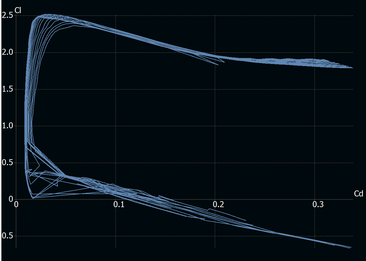
s1223.dat beside the XFLR5 sessions.Why this aerofoil
The Selig 1223 is a high-lift, high-camber section: it makes a great deal of lift at low speed and pays for it in drag. For a carrier that has to slow below 20 m/s to hand off a multirotor and does not have to be fast, that is the right trade. The design takes CL,max = 2.5 from it, which is what puts the stall speed at 18.9 m/s on a 6 m2 wing.
The drag polar beside it is the textbook one, parasite drag plus induced drag rising with the square of lift. At the design's own maximum lift coefficient it gives CD = 0.253, which reproduces the report exactly. Almost all of that is induced: flying at maximum lift is expensive, which is why 2.5 is a stall number and not a cruise number.
The wing as it was drawn and as it was analysed
The planform above is a rectangle at true scale, which is what the sizing script knows about the wing. These two are what the group actually drew and ran.

Whether it can fly the mission
PerformanceThe aircraft now has a weight, a wing and an engine. The question is whether the numbers that fall out of those reach the numbers the client asked for. Four of them matter: how far it goes, how long it stays up, how slowly it can fly, and how high it can climb before it runs out of thrust.
Thrust available falls with air density; thrust required does not. Where the two meet, climb stops. The absolute ceiling is where the rate of climb reaches zero and the service ceiling is the practical one, where it falls to half a metre per second and the aircraft can no longer usefully gain height.
Narration
01 The surplus
At sea level the engine has more thrust than the aircraft needs, and the surplus goes into climbing at about m/s. Everything after this is that surplus being spent.
02 Spending it
A kilometre up, density is % of its sea level value, and a propeller pushing on thinner air makes less thrust. The aircraft also has to fly faster to hold the same lift out of it, so the speed on the left is rising while the climb rate falls. At three kilometres, % and m/s. At five, % and m/s. The curve is close to a straight line, which is what a thrust surplus falling with density looks like.
03 The two ceilings
The service ceiling is the practical limit, where the climb rate falls to half a metre a second and the aircraft can no longer usefully gain height. km. The absolute ceiling is where the surplus reaches zero and the aircraft can only hold altitude. km. Both numbers rest on one assumption worth naming: the speed used at every altitude is the stall speed there, which is not a speed anything climbs at.
Against the brief
The senior engineer's six requirements, with what the design produced beside each one, and two numbers the design reports that the brief never asked for.
Range and endurance both clear the brief. The stall speed clears it by 1.1 m/s on the sizing sheet, which is thin, and the report's own summary says the simulated aircraft did not reach the target. The ceiling is the number with the least margin in the design and it is also the one computed on the shakiest assumption: the climb speed used at every altitude is the stall speed there, which is not how anything climbs.
Twelve numbers, and what it takes to steer them
The carrier, flyingThe sizing chapters produce a specification. This chapter is where it becomes an aircraft that moves. A rigid body in air has twelve state variables and no fewer: three positions, three body velocities, three attitude angles and three angular rates. Four control inputs act on them, elevator, aileron, rudder and throttle, and everything else, the forces and moments, is computed from the state each step and thrown away.
This is the weak half of the project, and it is worth being exact about why. The sizing chain above is a fixed point: it converges, it reproduces from the scripts to the last digit, and the number it lands on is the number the next revision starts from. The control work is not that. No loop on either vehicle was ever linearised. No gain margin or phase margin was computed for any of them. The gains were moved by hand until the traces looked acceptable, and the evidence for that is in the gains themselves, printed in chapter 06: thirteen values, and every one of them a round number. The one coupling that matters on a fixed-wing aircraft was abandoned rather than closed.
The model itself came with most of that already written. The aerodynamic
coefficients are the standard build-up, a base value plus a slope on angle of
attack plus a rate term plus a control-surface term, assembled into body-axis
force and moment coefficients and then into forces. What the template left blank
was the propulsion, marked in the file as
THRUST MODEL NEEDS TO BE COMPLETED HERE, and the four sections the
header names: setup, initial conditions, output and derivatives.
The thrust model that went in is the momentum form: a propeller accelerates a tube of air from the flight speed up to some higher speed set by the throttle, and the thrust is the difference of the two squared. It falls to zero when the aircraft is already flying as fast as the propeller can push, which is the behaviour of a fixed-pitch propeller.
The turn they could not make work
An aeroplane turns by rolling. Bank the wings and the lift vector tilts, its horizontal component pulls the aircraft round the corner, and its vertical component is now smaller than the weight, so you pull back to hold height. That coupling, roll to turn, pitch to hold altitude, is what a coordinated turn is, and it is where the longitudinal and lateral halves of the aircraft stop being independent.
The report is direct about what happened: "initial attempts to integrate fully coordinated altitude and heading control led to transient instability." The fallback was to command the heading, hold the wings close to level, and let the rudder yaw the aircraft flat onto the new heading. It works. It is also not how aircraft turn, and the report says what it costs: "A slight altitude loss occurs during the turn because the aircraft is not banking to produce a horizontal lift component."
That is the most valuable sentence in the report.
What the coursework did not ask for, and what the submission therefore does not have, is the thing that would have closed it. A coordinated turn is a coupled problem: you trim the aircraft at the turn condition, linearise the twelve states about that trim, and design the altitude and heading loops together against the coupled plant. Tuning them separately and hoping the coupling is weak is exactly what was done, and the altitude the report reports losing is the coupling arriving anyway. The instability was not bad luck. It was the predictable result of designing two loops for a plant in which they are not two loops.
The other vehicle
The surveyorThe carrier never lands at a site. What lands is a 3 kg quadrotor on a 0.44 m arm, dropped by parachute, carrying a half-kilogram sensor that finds animals from altitude and then needs the aircraft to come close and stay close. The mission it has to fly is written into the assignment as a sequence of trajectories, and the path-planning script that produces them was supplied. What was not supplied was any of the control.
The path is the output of the supplied plan_path.m,
recomputed here and drawn from above. One leg does not match the assignment prose
that describes it. which one, and why
Narration
01 Out, and holding
Off the ground and north to the holding position, 100 m out and 30.48 m up, which is the 100 ft the assignment specifies. A hundred seconds of climb, flown as a straight line in three dimensions rather than a climb then a translation. Ten seconds of hover at the holding position while the sensor suite finds something. This is the only leg with no commanded motion at all, and it is the one that shows whether the position loops hold station or drift.
02 The two animals
Animal A, walking due west. The assignment says 0.5 m/s for thirty seconds, which is 15 m. The supplied planner computes the endpoint from the number of steps rather than the elapsed time, so the leg it actually generates is 150 m. The plot bound in the supplied launcher is set to −200 m, which accommodates the longer leg, so the two supplied files agree with each other and not with the prose. Animal B, on a 10 m circle, one full revolution in a hundred seconds. This is the hardest leg for the controller: the position command is turning continuously, so the aircraft has to hold a steady lean into the curve while yawing to keep facing along it, and the yaw ramps through a full turn to do it.
03 Down
Down to the ground in a hundred seconds from 40 m, straight down with no lateral motion. The vertical loop is the one carrying the highest gains in the design, which is what you want on the axis where the ground is.
Nineteen blanks
The supplied launcher carries every control gain and every configuration value at
zero, under the comment TODO: please fill the following control parameters
out based on your own design. Filling them is the assignment. The table
below is that file before and after: the left column is what shipped, the right is
what was flown.
Read the right-hand column as a set before reading any row of it. Thirteen gains, and every one is a round number: 1, 0.5, 10, 5, 0.2, 0.1, 0.01. Nobody arrives at thirteen designed gains that all land on one significant figure. This is a set that was moved by hand until the simulation looked right, which is a legitimate way to get a demonstration flying and is not a control design.
One row is not a fill. K_i_psi, the integral term on yaw, is not in
the template's global declaration at all. It was added, which means the yaw loop
as designed is a PID where the template's skeleton assumed a PD. A quadrotor's yaw
is driven by the small difference between rotor drag torques and it holds a steady
bias readily; an integral term is the standard answer to a steady bias.
The control design is the weak part of this project, and it is not shown
The simulations ran, the demonstrations were produced and the deliverable was met. The loops behind them were tuned by hand against a plant nobody linearised, on a template whose gains all started at zero, to a standard that would not survive being looked at. The plots exist. They are not shown here, because a figure that cannot be defended is not evidence, it is decoration with a number on it.
What is worth keeping is the record of what failed and why, which is above: the coordinated turn that went unstable, the fallback that flew flat and lost altitude doing it, and the reason the instability was predictable rather than unlucky. That is the part of this work that transfers.
What was supplied and what was written
AuthorshipCoursework is a collaboration with whoever wrote the template. Every file below was compared against the distributed version byte for byte. Where a file was supplied complete it says so; where it was supplied with holes it says what was in the holes.
Supplied by the course
Written into it
The design itself is Group 10's. The mission plan, the choice of a turboprop, the aspect ratio, the aerofoil, the decision to fly the wing at 6 m2 rather than 3.94, and every conclusion in the report belong to the group and are stated that way throughout. The methods are textbook: Raymer for sizing, Beard and McLain for the flight model, standard PID for the loops. Nothing here is novel, and the value is in whether the chain closes, not in whether any link of it is new.
- 2024What the report states, or what a submitted script hardcodes.
- newComputed here and never stated in 2024. Two things only: the convergence walk, and the closure curves.
Reproducing the original calculation
The ledgerThe whole fixed-wing chain was ported to Python and checked against what the original wrote: twenty-six checks, each with a threshold argued from how precisely the report states its number, not chosen to pass. A report that writes 334.68 kg is checked to a hundredth; one that writes 0.8928 is checked to a ten-thousandth.
What the reproduction turned up
Porting a calculation is the most thorough reading of it there is, and it found seven things; reading the report against its own sizing sheet found an eighth. None of them is repaired in the source. Reproducing each as written is what makes the port a check rather than a rewrite.
What it shows
Nothing in this project is new. Raymer's sizing loop is forty years old, the six-degree-of-freedom model is out of a standard textbook, and the controllers are PID. What the work carries is that the chain closes end to end on one set of requirements: a client's mission becomes a gross weight, the gross weight becomes a wing, the wing becomes a performance envelope, and the envelope becomes an aircraft that flies the mission in a simulation whose every state is plotted.
It also records where it did not close. The wing area was chosen rather than derived. The coordinated turn went unstable and was replaced with a flat one that loses height. The ceiling rests on climbing at stall speed. The stall speed the sizing sheet meets is one the report's own summary says the simulation did not.
A conceptual design proposal, graded on vehicle weight, fuel weight and mission time. No aircraft was built and nothing here was flown outside a simulation.