UTIAS AER1410H · 2024 · coursework
Holes appear. This is the arithmetic that puts them there.
Density-based topology optimisation, from the textbook cantilever to a bracket, and one full pass of the optimiser opened up, stage by stage, so that "material migrates to where it carries load" can be checked against what the iteration does.
One iteration, all the way through
The mechanismAn optimiser that produces a good-looking truss is not evidence of anything until you can say what it computed. Below is a single pass of the loop, on the cantilever the coursework's own source defines, with every quantity drawn from the arrays that pass produced. The last stage hands its answer back to the first.
This is the published 88-line formulation executed here with every parameter stated, not a replay of the coursework's animation, whose own penal and rmin were never written down.
The pass
01 What it starts from
A density for every element: 1 is solid, 0 is void, and everything between is the fiction that makes the problem differentiable. Stiffness is not proportional to density; it is ρp with p = 3, so an element at half density buys an eighth of the stiffness for half the material budget. Intermediate density is deliberately made a bad deal, which is what drives the field to black and white.
02 What it computes
Assemble the global stiffness from those densities and solve K u = F once. Ten thousand degrees of freedom, one linear solve; this is the expensive stage. Each element's own strain energy ueᵀ k₀ ue falls out of that solution. It is how hard this element is working. Summed with the density weighting it is the compliance: the objective. Lower means stiffer.
03 Which way to move
The derivative of compliance with respect to each density is −p ρp−1 ueᵀ k₀ ue. It is negative everywhere, which says adding material anywhere would help, so the volume constraint is what makes this a problem at all. Filtered over a radius of three elements. Without this the answer is a checkerboard: alternating solid and void elements that the finite-element model scores as artificially stiff. The filter is not smoothing for looks, it is what makes the answer mesh-independent.
04 The move, and the next field
The optimality-criteria update: raise density where the filtered sensitivity is large, lower it where it is small, and bisect on a Lagrange multiplier until the volume comes out exactly at the budget. No element moves more than 0.2 in one step. Here is what moved. Red gains material, blue loses it, and the two integrate to zero because the constraint binds. This is the answer to "why do holes appear". Nothing removes material: the budget is fixed, so material arriving somewhere is material leaving somewhere else. And then it goes round again, sixty times.
Making the middle a bad deal
The true problem is discrete: every element is solid or void, and that is a combinatorial problem with 5 000 binary variables. SIMP relaxes it by letting density run continuously from 0 to 1 and interpolating the element's Young's modulus as E(ρ) = Emin + ρp(E₀ − Emin), which makes the problem differentiable and therefore solvable by gradient methods.
The relaxation is only useful if the answer comes back discrete, and p is what forces that. At p = 1 stiffness is proportional to material and a half-dense element is a fair trade; the optimiser has no reason to commit and returns a grey mist. At p = 3 that element buys an eighth of the stiffness for half the budget, so grey is strictly worse than the same material concentrated somewhere. The penalty is not a physical model of anything. It is a device that makes the continuous answer land on the discrete one, and Emin is a small floor that keeps the stiffness matrix invertible where density goes to zero.
One solve, all five thousand derivatives
A gradient with respect to 5 000 variables would normally cost something close to 5 000 solves, or one adjoint solve if the problem is set up for it. Minimum compliance costs neither, and the reason is worth stating. The objective c = Fᵀu with Ku = F and K symmetric is self-adjoint: the adjoint vector turns out to be the displacement field itself.
So the derivative falls out of the solve already done: ∂c/∂ρe = −p ρep−1 (E₀ − Emin) ueᵀ k₀ ue, one small element-level product per element. That is why a topology optimiser can afford sixty iterations on a laptop, and it is a property of this objective rather than of the method: a stress-constrained or compliant-mechanism problem is not self-adjoint and pays for its gradient.
Two filters, and they are not the same idea
Left alone, the optimiser produces a checkerboard: alternating solid and void elements. This is not a physical structure; it is an artefact of the four-node element, which models that pattern as stiffer than it can possibly be, so the optimiser is correctly exploiting a bug in its own analysis.
The sensitivity filter replaces each element's derivative by a distance-weighted average over a radius of rmin elements. It is a heuristic: the filtered derivative is not the derivative of any objective anyone has written down, and it works anyway, which is why it became standard. The density filter instead averages the design field itself and differentiates through the averaging, so it is consistent; there is a real objective being minimised. The comparison further down runs the same problem with only that switch changed: the heuristic gets to a lower compliance in fewer iterations, and the consistent one is the one whose answer means something.
The multiplier is the price of material
The update is not a step along the gradient. Optimality criteria comes from the KKT conditions of this specific problem: at the optimum, every element that is neither at 0 nor at 1 has the same ratio of stiffness gained to volume spent. Call that common ratio λ; it is the Lagrange multiplier on the volume constraint, and it is the shadow price of material.
Guess λ, and each element's new density follows in closed form: raise it where its sensitivity beats the price, lower it where it does not, clipped to [0,1] and to a move limit of 0.2 so no element can flip in one step. The resulting volume is monotone in λ, so a bisection of thirty-odd evaluations lands on the price at which the budget is spent exactly. In the run below the measured volume fraction is 0.667 on the first frame and 0.499 on the second, so the constraint is not yet binding there; from the third frame it holds at 0.399 and never moves again.
A length scale has to come from somewhere
Without a filter, refining the mesh does not converge the design: it produces a different design with finer members, because nothing in the formulation says how thin a member is allowed to be. More elements simply buy more places to put thinner structure, and the compliance keeps improving.
The filter radius is what supplies the missing length scale, and here it is declared in elements: rmin = 3.0 on a 100 × 50 grid. Double the mesh without doubling rmin and the physical filter radius halves, so the answer changes. That is a real limitation of the result shown here: the fields are converged for this discretisation, and no mesh-independence study was run.
Every term above, in the order the course builds them
Reference · open what you needThe loop is short enough to watch and long enough to hide five separate ideas, each of which exists because the one before it created a problem. This is the dependency chain, in the order AER1410 teaches it.
Every entry answers the same four questions: what it is, why it exists at all, why it matters here, and what changes because of it. Three names it does not stop to define, because they are the subject rather than the method: SIMP is Solid Isotropic Material with Penalization, the formulation this whole page is about; the half-MBB beam is the standard test case Sigmund's code ships set up for, an aircraft floor-beam problem named for Messerschmitt-Bölkow-Blohm; and Ku = F is the finite element system, stiffness times displacement equals load.
Nineteen frames the optimiser wrote about itself
The coursework's own runThese are not renders of the result. The coursework's own script opens a VideoWriter and calls getframe inside the optimisation loop, so each frame is a design field the optimiser was holding at the moment it wrote it. The grid, 100 × 50, was measured back out of the frames by FFT of the image gradient, because it is not recorded anywhere in the tree.
The volume fraction measures 0.667 on the first frame, 0.499 on the second, and lands on 0.40 by the third, where it never moves again: the constraint binding exactly, and why the structure can only reorganise from here rather than grow.
One comparison, and then stop
The same 200 × 40 problem run twice, changing only the filter. The sensitivity filter reaches a lower final compliance in fewer iterations; the density filter takes 100 more iterations to arrive somewhere worse on this objective, though it is the one with a physical meaning, since it filters the design variable rather than its derivative.
What was provided, and what was not
AuthorshipThis lineage is one of the most widely taught pieces of code in structural optimisation, and the assignment was designed around that: the point was not to write an optimiser, it was to understand one well enough to pose a problem to it and to read what came back.
The three modifications are small and they are the whole assignment. Sigmund's code ships set up for the half-MBB beam with a symmetry plane. Turning it into this cantilever means replacing the support set, moving the load, and introducing a passive region the optimiser is forbidden to fill, which is how a real bolt hole or a clearance envelope enters a topology problem.
| part | where it comes from |
|---|---|
| SIMP interpolation, FE solve, OC update, filter | provided |
| Supports: the whole left edge clamped, replacing the half-MBB symmetry condition | P1_r3.m:125 |
| Load: a single downward point load on the right edge | P1_r3.m:125 |
| Passive region the optimiser may not fill | P1_r3.m:14–29 |
| Frame capture inside the loop | P1_r3.m:36–39, 76–78 |
| Filter comparison: the same problem twice, changing only ft | Problem Set 7/Q1 |
| The bracket case, its load estimates and the polyNURBS fit | assignment work |
Problem Set 4 is a different case: top.m:100 and top99neo.m:31–32 leave Sigmund's half-MBB supports in place, so nothing from it is shown here.
The same method on a bracket somebody has to machine
What it was pointed atThe second half of the course applied it to the leading-edge slat bracket of a Zenith STOL CH 750: four fastener locations, a multi-directional load case, and a downstream shape somebody has to machine. The raw density iso-level is not a manufacturable surface; the polyNURBS fit is the step that turns the method into an engineering result rather than a picture.
The topology is identical before and after the fit: same two triangular voids, same brace.
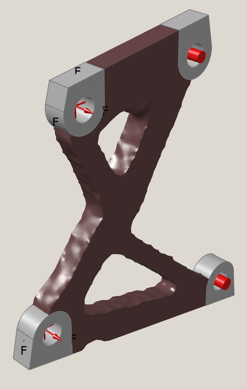
volume fraction 0.35, iso-level surface
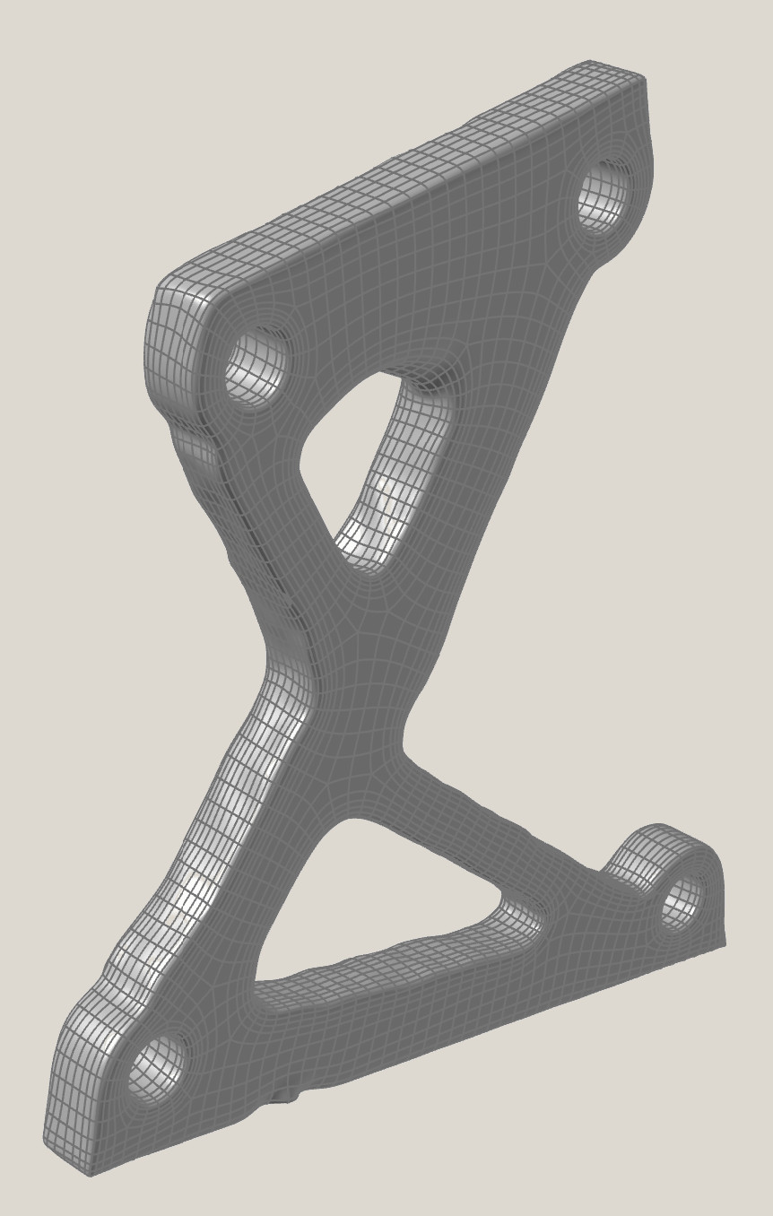
same run, machinable surface
The same optimiser, on the course's other problems
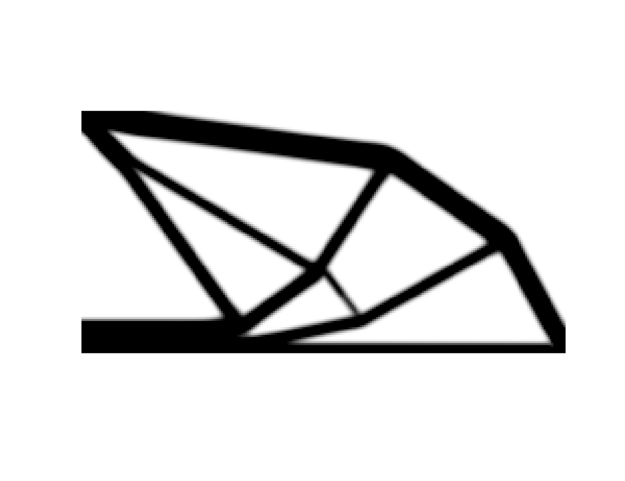
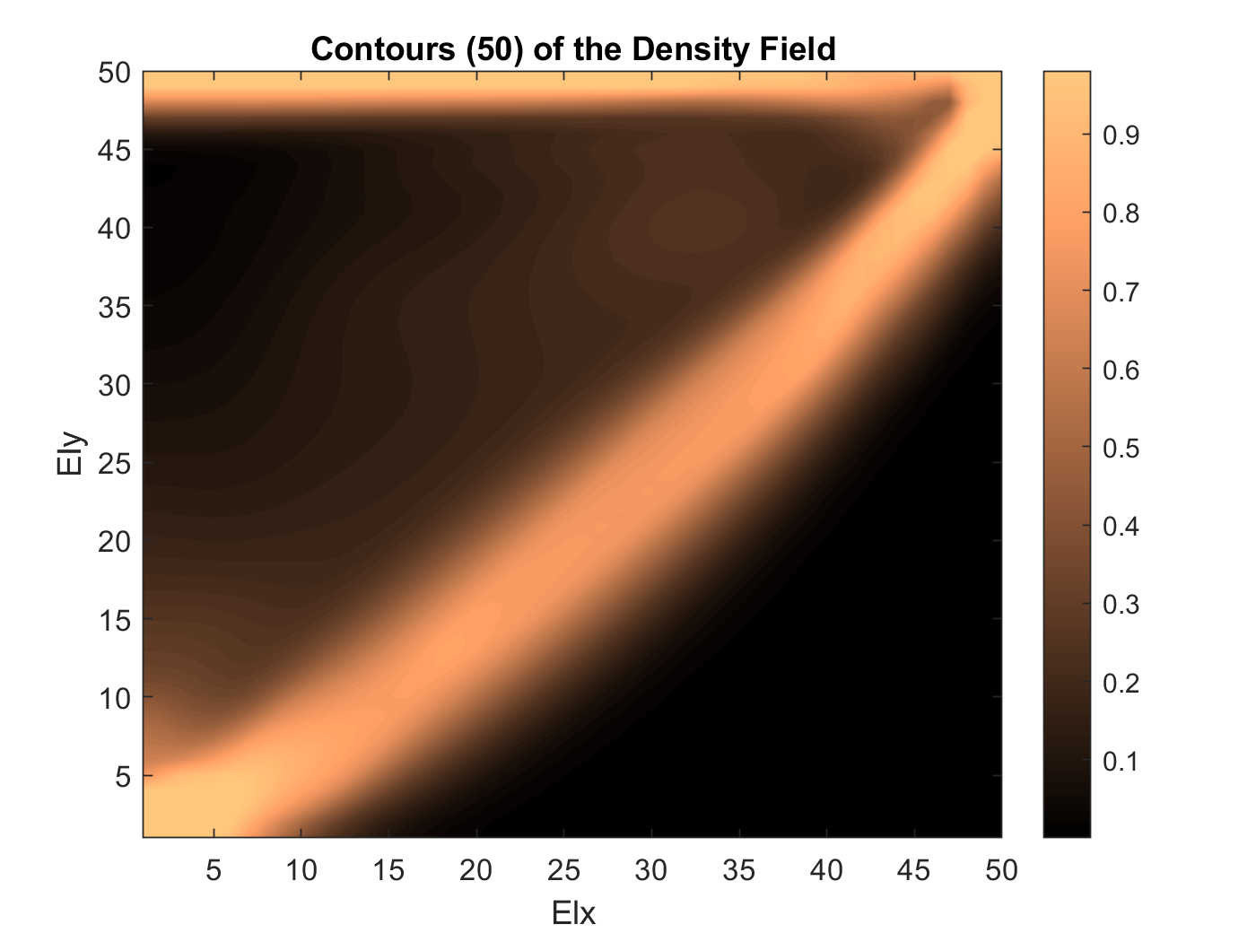
The chapters above follow one problem all the way through. These are two more the same code produced, kept because they show the two shapes a topology result comes in: a discrete truss and a continuous density field.
What this does not establish
- Coursework. Two-dimensional, compliance objective, SIMP with a linear-elastic solve. No stress constraint, no buckling, no fatigue.
- The stage-by-stage pass at the top is a reconstruction of the mechanism, not of the coursework run: it uses the published 88-line formulation with stated parameters, because the animation's own penal and rmin are not recorded anywhere in the tree.
- The nineteen frames are evidence of what that run produced. Their grid and volume fraction are measured back from the images rather than read from a log, and the saved still beside them is named for a different call.
- The bracket load cases are estimates from STOL flight profiles, not measured loads.
- A lower compliance is not a better part. The filter comparison is one objective on one problem.