Human control of flight systems · identifying a pilot from fifteen sine waves

01

What the person was doing

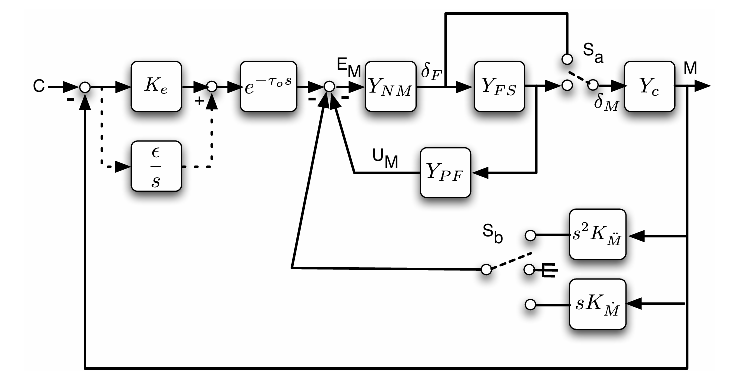
The experiment

Before any frequency response, the task. The simulator flew a commuter aircraft at 5 000 ft and Mach 0.2. A target sat at zero pitch attitude and the pilot's job was to keep the nose on it. While they flew, a disturbance signal was added to the control column ahead of the aircraft, so the aeroplane kept getting pushed off the target and the pilot kept putting it back. That is a disturbance rejection task, and the loop below is the one the assignment draws.

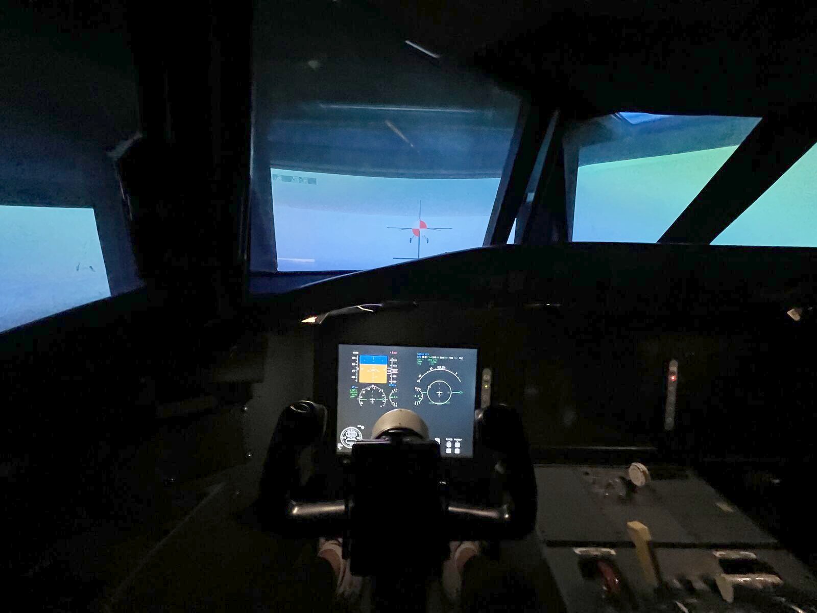
The UTIAS flight research simulator cab from the pilot's seat: out-the-window visual with a target aircraft ahead, a lit glass PFD and MFD on the centre console, the yoke in the foreground and the throttle quadrant to the right. — 2024 The seat the four recordings were flown from, photographed in the darkened cab. The target aircraft ahead is the thing the nose is being held on; the glass panel below it is the display the pilot was reading; the yoke is the column whose deflection is row 5 of the data matrix, and the disturbance was being added to it while this was taken.

Each run is a matrix of 13 rows by about 25 000 samples at 180 Hz, roughly 141 seconds of flying. The identification uses three of those rows and builds a fourth. The target was at zero attitude, which is what makes the error simply the negative of the pitch: there is no separate command signal to subtract.

Two things were changed between runs and nothing else was. The motion platform was switched off or on, and the control column's feel system was set to a high or a low force gradient, meaning how hard the column pushes back per inch of deflection. Four combinations, four recordings, and the same disturbance signal in each.

I was the pilot in all four recordings, and the analysis is mine. The assignment names each file by the student's initials, and these are the MS files. That is the most interesting fact in the project and it is also its tightest limit: one person, one afternoon, one vehicle model.

02

A time trace answers the wrong question

From seconds to frequencies

Here are twenty seconds of the run the 2024 coursework analysed. The disturbance pushes, the column answers, the nose wanders. It is obviously a person working, and it is almost useless as evidence, because everything a pilot does at every rate is superimposed in it. A slow correction and a fast twitch land in the same wiggle.

The way out is the disturbance itself. It was not noise. It was built as a sum of fifteen sinusoids at chosen rates, listed in the assignment as periods per minute: 1, 2, 3, 4, 5, 7, 9, 13, 18, 23, 33, 43, 58, 73 and 131. Transform the recording and it is not a spectrum at all, it is a comb.

Narration

01 Why sinusoids and not noise

Noise would drive every frequency a little. A sum of fifteen sinusoids drives fifteen frequencies a lot and everything else not at all, so at those fifteen the pilot's output can be attributed to the input with almost no ambiguity, and Welch's method has enough repeats of each sine in the window to average the estimate down. The amplitudes are not equal: the fastest component, 131 cycles per minute, carries the largest of the set at in.

02 The floor between the lines is the person

The disturbance stands dB above its own floor. The column stands dB above its floor. That difference is remnant: the part of what the pilot did that was not a linear response to what they could see. It is not measurement noise and it does not average away. It is the reason a pilot is described by a linear model only at the frequencies where the input is loud enough to dominate it.

03 Fifteen points

Fifteen points across two decades. Between them the identification has nothing to say, and the next chapter measures exactly how little. It is also why the crossover frequency later has to be interpolated: 0 dB is not one of the fifteen.

03

Divide the answer by its own cause

Identification

At each of those fifteen frequencies the input is known, so the response can be divided by it. For a disturbance rejection task the estimator the course derives is a ratio of cross spectral densities between the disturbance and two other signals: Y_p(jω) = Φ_do / Φ_de, the disturbance against the pilot's output over the disturbance against the error. It is chosen because it is the ratio that minimises the effect of the pilot's own unrepeatable behaviour on the answer.

That last part has a name. Everything a pilot does that is not a linear response to what they can see is called remnant, and it is not small. In the column spectrum above it is the floor between the fifteen lines. The estimator cannot remove it, but it can be measured, and the course's goodness of fit parameter ρ² is exactly that measurement: how much of the pilot's output at a given frequency is linearly attributable to the disturbance.

04

The loop the pilot closed

The instrument

One object, six views, all of them the same two panels: how much a signal is amplified at each rate, and how far behind it comes out. The first three views build the loop from its parts. The fourth reads the two numbers every stability argument in this project rests on. The last two are used by the chapters below.

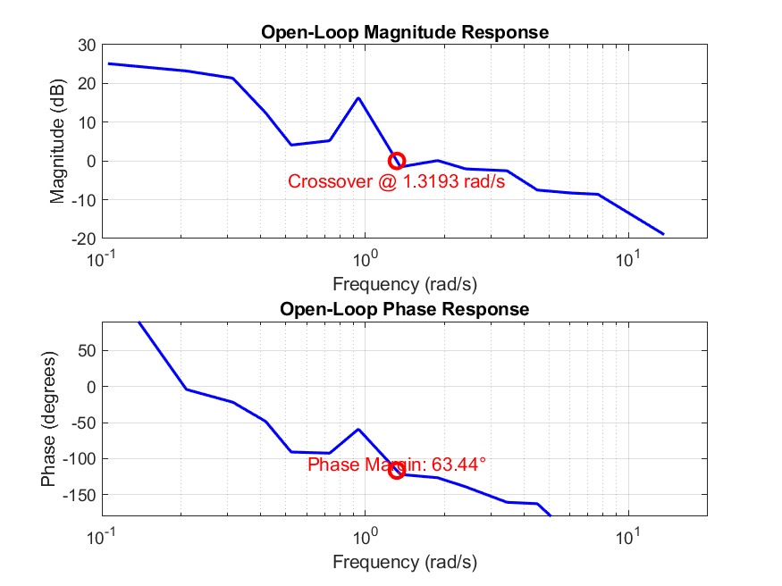
Read the magnitude panel as how much nose you get per inch of column at each rate, in decibels, and the phase panel as how far behind the nose arrives, in degrees. Both are drawn against a logarithmic frequency axis, which is the only axis on which a decade of slow behaviour and a decade of fast behaviour get equal room.

Frequency

Narration

01 The two things it multiplies

Start with the aeroplane, because the pilot did not choose it. This is the transfer function from column inches to pitch radians that the assignment hands out, and it is the same in all four recordings. Two lightly damped pairs of poles, a slope steepening past about 1 rad/s, and phase already through −90 degrees before anything human is added. given by the assignment, not measured Now the measurement. Each dot is one driven frequency, and its height is the ratio of two cross spectral densities computed from two minutes of the recording. There are fifteen dots because there are fifteen frequencies where the input was known; the line joining them is drawn, not measured. The shape is a person compensating: gain is high at low frequency, because a slow drift off target is easy to see and worth correcting hard, and it falls away at high frequency, because a human cannot follow a two hertz wobble and stops trying. The lowest driven frequency sits above the top of the phase panel, and MATLAB's own figure clipped it too, at +90 degrees. Yp = Φdo / Φde, from 21 600 samples

02 The loop, and its two numbers

The pilot's response times the aircraft's response is the open loop: what one trip around the circle does to a signal. This is the quantity every stability statement on the page is about, and it is the product of one thing that was given and one thing that was measured. The 2024 figure in chapter 08 draws exactly this curve, with the same fifteen corners. L = Yp · Yc Crossover is the frequency where the loop gain passes through one, drawn here as 0 dB. Below it the loop is strong and errors get corrected; above it the loop is weak and errors mostly get through. Phase margin is read at that same frequency in the panel below: how far the phase is from −180 degrees, where a correction comes back around the loop perfectly wrong and the loop oscillates. The vertical bar in the phase panel is the margin, drawn to scale. Both come from one frequency, which is why they are always quoted as a pair.

03 The other three runs, and four models

The same construction applied to the other three files. The two motion runs sit visibly to the right: the whole loop moved up in frequency. Chapter 05 takes this apart. three of these four were never analysed in 2024 Four model open loops drawn over the measured one. None of them was fitted to this pilot, and chapter 06 says what each one is made of and which of its numbers were chosen rather than produced. The optimal control model is absent from this view because it could not be recomputed here; its two crossover frequencies appear on the axis in chapter 06 as reported values.the crossover models, the precision model, the structural model

05

The three recordings nobody analysed

A new question, from preserved data

The 2024 assignment asked for one file: XX-NM-HPNZ.mat, no motion, high force gradient. That is the one that was analysed, and the analysis was correct for the question asked. The other three recordings were flown on the same afternoon, written to disk, submitted with the assignment, and never opened again.

They are still there. Running the identical verified pipeline over all four is the only computation here that is not a reproduction of anything, and every number it produces is marked new. It is a question the preserved data can answer and the coursework never asked: what did turning the motion platform on do to this pilot?

Four recordings, one pipeline
Condition	ω_c rad/s	Phase margin deg	RMS error deg	RMS column in	Mean ρ²

The two stories are not the same story

These are the changes observed in these four runs, not an effect established over a population of pilots. A second pilot could reverse any of it.

06

Four models that claim to predict a pilot

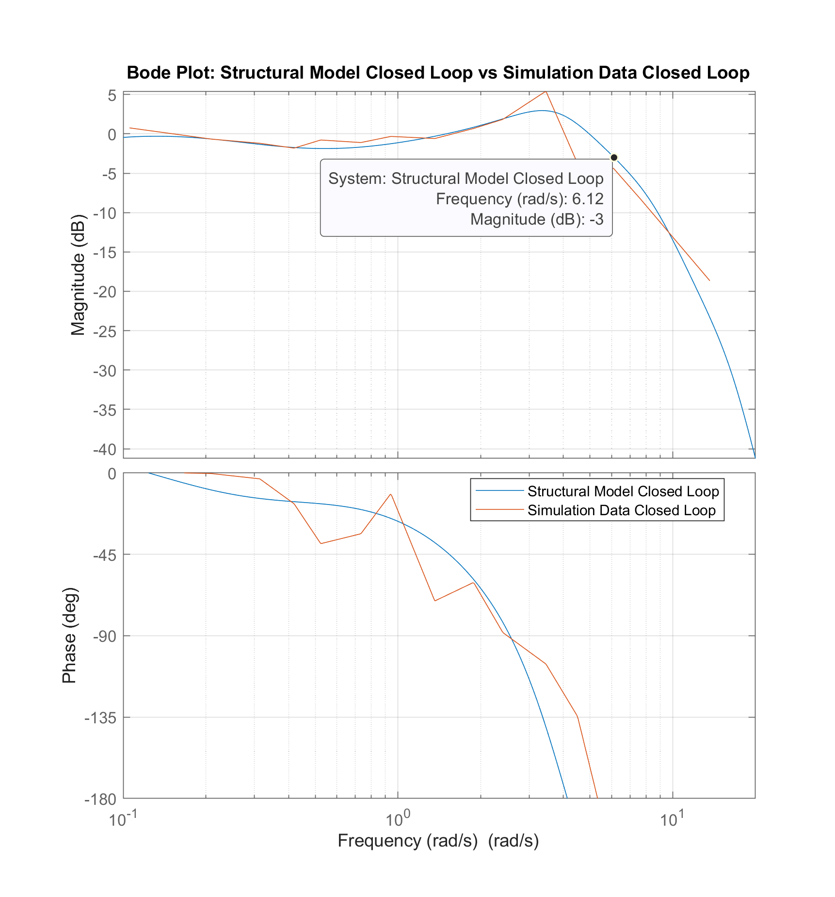
Prediction against measurement

Human control has a century of models that will tell you what crossover frequency a pilot ought to adopt for a given vehicle, without ever looking at a pilot. The coursework built four of them for this aircraft. Below, all of them sit on one axis with the four measurements, and each is marked by what kind of number it is: a genuine output of the model, or a value a parameter was chosen to produce.

The Hess structural pilot model as a block diagram: a command summed against the vehicle output, an error gain K_e with a parallel integral trim path, a delay, the neuromuscular block Y_NM, the force-sense block Y_FS with a proprioceptive feedback Y_PF around it, and two switched vestibular feedback paths carrying the second and first derivatives of the vehicle motion. — course The structural model as the course draws it. Follow the loop: the error is scaled by K_e, delayed, and passed through the neuromuscular block; the force-sense block drives the column and feeds a proprioceptive signal U_M back inside the delay; the two switches at the right are the motion cues, and throwing them is what "motion on" means to this model. **The gain at the far left is the one that was chosen to place crossover at 2 rad/s**, which is why the model's crossover is an input to it and not a result from it. This diagram is the course's, not a redrawing.

The measurement is not free of choices either: the window, the overlap, the start time and the interpolation between data points are all decisions, and one of them is worth twelve degrees of phase margin. What the measurement did not require was a form for the human. No table of pilot delays was consulted, no lead time constant was selected, no cost function was assumed. That is the difference between it and every other entry on the axis above.

The 2024 MATLAB figure comparing the structural model's closed-loop frequency response against the closed loop formed from the measured pilot, magnitude above and phase below. — 2024 The structural model's closed loop against the one built from the measured pilot, as MATLAB drew it in 2024. This is the comparison the model chapter is arguing about. The two closed loops agreeing in the mid band is not independent evidence for the model, because the gain that sets where they agree was chosen to make them.

07

What it costs the person to fly it

Handling qualities

A model that is asked about workload

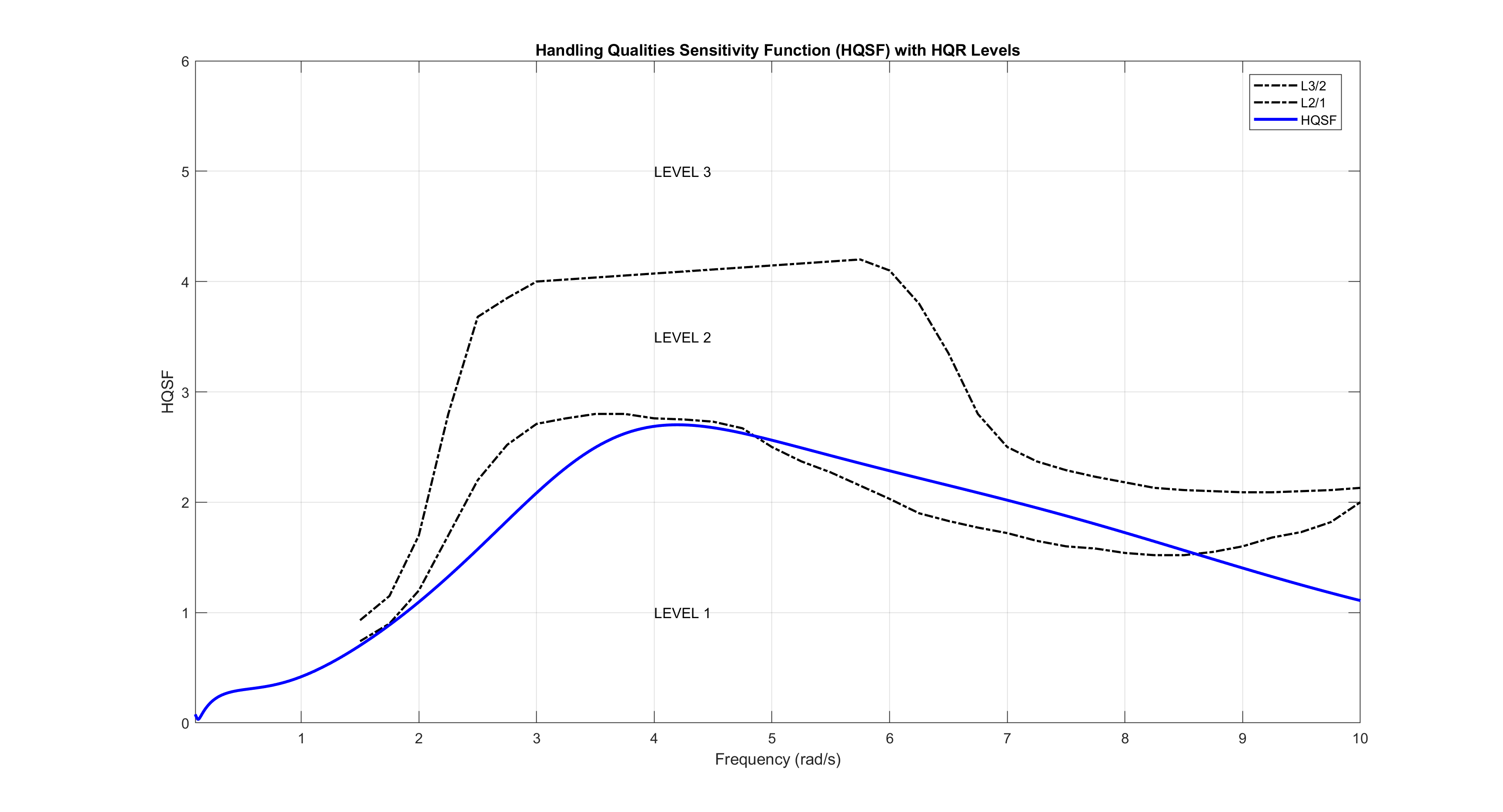
Stability margins say whether a loop holds together. Handling qualities ask a different question: what does holding it together cost the person. The course's handling quality sensitivity function reads the effort the structural model's proprioceptive path has to produce for a given amount of vehicle response, and the two dashed curves are the instructor's own digitised boundaries between Level 1, Level 2 and Level 3.

This is a model result, not a measurement. It inherits every parameter the structural model chose by hand, and the boundaries themselves come from a data file the course supplied. It says what the model implies about workload; it does not say what the pilot experienced.

The 2024 MATLAB figure of the handling qualities sensitivity function against frequency, with the Level 3 to 2 and Level 2 to 1 boundaries dash-dotted and the three level regions labelled. — 2024 The same quantity as MATLAB drew it, for the high force gradient case. Compare it with the panel above, which is the same computation redrawn from the model. The boundaries are the course's digitised curves in both.

08

Reproducing the original calculation

What the port found

Every number above came out of a Python port of the 2024 MATLAB analysis, checked against what the original wrote. Twenty-two checks, with thresholds argued from how precisely each source states its number rather than chosen to pass. Two of them turned up things the 2024 report does not say about itself. Neither has been repaired in the original; both are reproduced as written and described here.

The 2024 MATLAB figure of the open loop: a magnitude panel in decibels and a phase panel in degrees, both against log frequency, with a red circle at the crossover and the text Crossover at 1.3193 radians per second and Phase Margin 63.44 degrees printed into the image. — 2024 The evidence the whole port is checked against. MATLAB printed its own answer into the picture, so the two numbers survived without depending on anyone's memory. Note the straight segments: the curve is fifteen measured points joined by the interpolation that `bode()` performs, which is the detail that had to be identified rather than assumed.

Check	Recomputed	2024 source	Tolerance	Why that tolerance

What survives from 2024 is not a conclusion about pilots. It is a method and a recording.

Scope

n = 1. One pilot, four runs, one afternoon, one vehicle model. Every difference between conditions is a difference observed in these recordings and nothing more. No population effect is claimed and none can be.
I was the pilot and I did the analysis, which removes any question about whose data this is and adds every question about a single subject knowing what the experiment was testing.
The identification is exact only at fifteen frequencies. Crossover falls between two of them in all four runs, so the headline numbers are interpolated across a measured gap.
The optimal control model's two crossover frequencies are quoted from the 2024 report and are not reproduced here. They come from a Simulink model driven by fmincon, and were not ported.
The Hess structural model's 2 rad/s crossover is not evidence of anything: a gain was set to put it there. Its phase margin, gain margin, bandwidth and resonance are, and those are what the port checks.
Handling quality levels are a model output read against boundary curves the course supplied. They are not a pilot rating and nobody rated this aircraft.
Two discrepancies in the 2024 report are reproduced rather than corrected. The original coursework has not been edited.