Independent · ongoing · flagship
Building a solver is one thing; knowing whether it is right is the other.
CFDLab is a Python companion to the Lomax–Pulliam–Zingg curriculum: analytical probes, three structurally different quasi-1-D Euler solvers, and baselines pinned by MD5 under one local gate, so the gate fails when a number moves. Two of the three are measured on this page. ARC1D is the central-difference solver with JST artificial dissipation; upwind1d is the characteristic-decomposition solver, Roe with MUSCL reconstruction.
Two solvers, the same shock tube, the same grid spacing, the same final time. One adds a scalar dissipation term to a central scheme; the other decomposes the flux into characteristic waves and upwinds each one separately. Both are stable. Both conserve mass, momentum and energy. Both produce a plausible picture.
They are not equally right, and the place where they differ most is not the shock; it is the contact discontinuity, the one wave that carries no pressure jump and therefore gives a pressure-driven dissipation term nothing to lock onto. What follows is one measurement of that difference, taken from the arrays the repository commits.
The case
- p left
- 100 000 Pa
- p right
- 10 000 Pa
- ρ left
- 1.000 kg/m³
- ρ right
- 0.125 kg/m³
- diaphragm
- x = 5.0 m
- final time
- 6.1 ms
- γ
- 1.4
- Δx
- 0.025 m
If none of those words are familiar yet, chapter 03 builds them one at a time, in the order they depend on each other, against this same experiment. Nothing below assumes you read it.
The experiment, from a burst diaphragm to a counted width
The measurementA tube closed at both ends, a diaphragm at the midpoint, and a pressure ratio of ten across it. Six milliseconds after the diaphragm bursts, three waves are running and one of them is the subject.
Narration
01 The problem
Ten metres of tube, closed at both ends, divided by a diaphragm at the five-metre mark. At t = 0 the diaphragm is removed, and a pressure ratio of ten has to resolve itself into whatever waves the Euler equations permit.
02 What the physics does
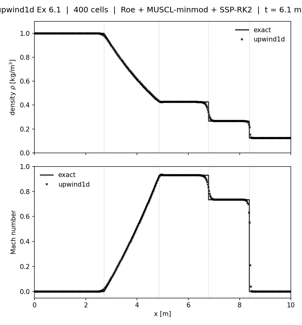
Six milliseconds later the closed-form solution has three distinct waves in it, and only one of them is a shock. Running left, an expansion fan: a smooth, continuous acceleration spread over about two metres by 6.1 ms. Running right at 554 m/s, a shock: a genuine discontinuity, compressive, self-steepening. Between them, moving at the flow speed itself, the contact discontinuity.
The contact is the odd one out, and this is the whole point: switch the plotted quantity to pressure and the contact vanishes. Density jumps across it by a factor of 1.6; pressure does not change at all.
03 What each scheme does with it
ARC1D adds a scalar artificial-dissipation term to a central difference and runs 150 implicit steps at Courant 1; the shock comes out six cells wide between the 10 and 90 % points of its jump. upwind1d splits the flux difference into the three characteristic fields and upwinds each separately, with MUSCL-minmod reconstruction and adaptive SSP-RK2 at CFL 0.8. On this scale the two are almost indistinguishable, which is exactly the problem: a plausible picture is not evidence.
04 Where they differ
One metre of tube around the contact, and the difference that was invisible at full scale is now the only thing in the frame. Inside a fixed window, the repository counts the cells whose density sits outside ±2 % of both bounding plateaus. Twenty-six cells for JST, sixteen for Roe + MUSCL, counted from the rarefaction tail to the exact shock position, so the shock's upstream half is in the count; the gap is concentrated at the contact. A factor of 1.6, and neither scheme holds the contact within one cell.
Why the contact is the hard one
The argumentThe chart above shows a difference. The reason is a property of the equations, not of either implementation, which is why it was predictable before the counting was done.
The mechanism, and why it was predictable
Open where you need it
A shock is compressive. The characteristic speeds behind it exceed those ahead of it, so the profile steepens on its own and a scheme's dissipation is continually fought by the physics. Whatever smearing the numerics add, the nonlinearity pushes back. The result is that a shock stays narrow: between the 10 and 90 % points of its jump, Roe holds it in three cells here and JST in six.
A contact is linearly degenerate. Its characteristic field is the one whose speed is the flow velocity itself, and the wave speed does not change across the wave. Nothing steepens. There is no mechanism at all to oppose numerical diffusion, so whatever a scheme smears on step one it keeps, and adds to, every step after.
Scalar artificial dissipation makes the problem worse in a specific way. JST's switch is built from a normalised second difference of pressure, because pressure is what detects a shock. Across a contact the pressure is constant, so the sensor reads zero, the higher-order term is not switched off, and the background fourth-difference dissipation smooths the density jump unopposed.
Roe's flux-difference splitting decomposes the jump between neighbouring cells into the three characteristic fields and applies upwind dissipation to each one on its own. The contact is one of those fields. It gets dissipation proportional to |λ₂| = |u| rather than to the largest wave speed in the cell, which is roughly a factor of (|u| + a)/|u| less. That is the mechanism the measurement above is detecting.
The JST pressure switch
The second-difference coefficient is ε⁽²⁾ⱼ = κ⁽²⁾ · max(νⱼ₋₁, νⱼ, νⱼ₊₁) with the sensor νⱼ = |pⱼ₊₁ − 2pⱼ + pⱼ₋₁| / (pⱼ₊₁ + 2pⱼ + pⱼ₋₁). It is a normalised second derivative of pressure: large at a shock, and identically zero anywhere pressure is linear, which includes a contact, where pressure is not merely linear but constant.
The fourth-difference term ε⁽⁴⁾ⱼ = max(0, κ⁽⁴⁾ − ε⁽²⁾ⱼ) exists to damp odd–even decoupling in smooth regions. At the contact ε⁽²⁾ = 0, so ε⁽⁴⁾ is at full strength and acts on a jump it was never designed to see. The smearing is not a bug in the implementation; it is what this discretisation does.
Where the factor comes from
Roe's flux is F½ = ½(Fᴸ + Fᴿ) − ½ Σₖ |λ̃ₖ| α̃ₖ r̃ₖ, with the wave strengths α̃ₖ obtained by projecting the state jump onto the eigenvectors of the Roe-averaged Jacobian. The dissipation applied to field k scales with |λ̃ₖ|: that field's own speed.
A scalar scheme cannot do this. It has one dissipation coefficient per cell, and for stability it must be sized by the fastest wave, |u| + a. At the contact the physically correct amount is set by |u| = 293 m/s while the sound speed there is a ≈ 313 m/s, so the scalar scheme applies roughly (293 + 313)/293 ≈ 2.1× the dissipation the wave calls for. The measured cell counts differ by 1.6.
MUSCL, and why minmod
First-order upwinding is monotone but heavily diffusive. MUSCL raises the order by reconstructing a linear profile inside each cell before solving the Riemann problem at the face, which recovers second-order accuracy in smooth regions and, unlimited, produces oscillations at every discontinuity (Godunov's theorem: no linear scheme above first order is monotone).
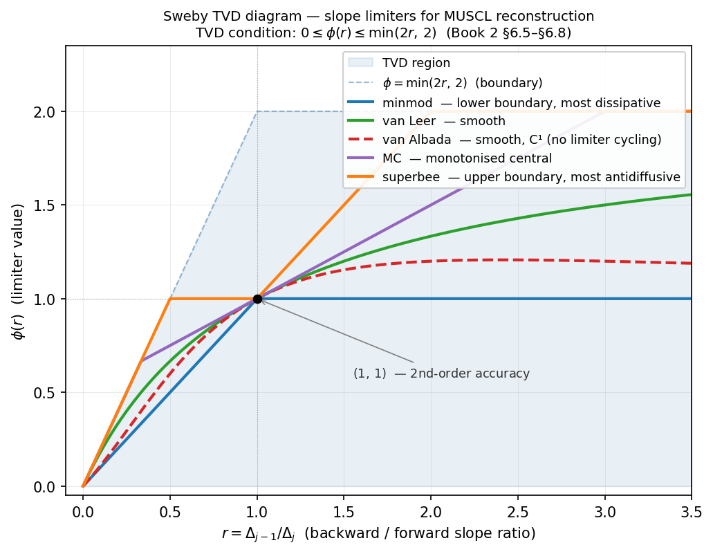
The limiter is what buys monotonicity back. Minmod takes the smaller of the two neighbouring slopes and zero if they disagree in sign, which is the most diffusive of the standard TVD limiters: the conservative choice. A less diffusive limiter would sharpen the contact further; that the most diffusive TVD limiter already beats scalar dissipation by 1.6 is the point.
Verification, not validation
Verification asks whether the code solves the equations it claims to solve. Validation asks whether those equations describe reality. This comparison is entirely the first: the reference is an exact closed-form solution of the same Euler equations, not a wind tunnel, so there is no modelling error anywhere in the comparison and every discrepancy is discretisation.
That is what makes the number meaningful and also what bounds it. It says nothing about whether the Euler equations are the right model for anything: only that, for a problem with a known answer, one discretisation is measurably closer to it than the other.
One number per cell, per equation
A finite-volume cell does not store the solution at a point. It stores the average of the conserved quantities over the cell's own width: here three numbers per cell, ρ̄, ρu and ρE, over Δx = 0.025 m. Nothing finer than that exists inside the computation.
That is why a count of sixteen cells in transition is a statement about information and not about drawing. A jump that truly occupies zero width has been replaced by a staircase of averages, and the only question a scheme can answer is how many stairs it takes to climb. Two or three is as good as a finite-volume method gets; sixteen and twenty-six are what these two schemes spend between the fan and the shock, most of it on a wave with nothing to hold it together.
Central, plus a term that is not
The scheme's flux is a plain arithmetic average of the two neighbouring states; that is the central part, and on its own it is second-order accurate and unconditionally unstable for this system: it has no mechanism to damp the odd–even mode, and none to tell an upstream cell from a downstream one.
JST keeps that central flux and adds an explicit dissipation term beside it, tuned by two coefficients. The name records the construction, not the behaviour: the discretisation is central, and the stability comes from something bolted on next to it. An upwind scheme has no such term because the dissipation is already inside its flux, which is exactly what lets Roe apportion it wave by wave and JST not.
Conservation is a property of the update, not of the physics
Both schemes advance a cell by differencing the two fluxes on its faces. Sum that over every cell and each interior face appears twice with opposite signs, so the total of each conserved quantity changes only through the two ends of the tube. The domain is closed, so the totals do not change at all: to machine precision, on any mesh, at any accuracy.
Discretise the non-conservative form instead: write the equations in terms of ρ, u and p and difference those, and the cancellation is gone. The scheme still converges, and it converges to a shock moving at the wrong speed, because the Rankine–Hugoniot condition that fixes that speed is a statement about fluxes. It is the one error a finer mesh does not fix.
Every term above, in the order it depends on the one before it
Reference · open what you needThe argument is finished. This is the apparatus underneath it: the dependency chain the experiment rests on, each term only meaningful once the one above it is. Open a term where it is unfamiliar.
Each entry answers the same five questions: what it is, why it exists at all, why it matters here, what physically or numerically changes because of it, and where to see it in this result. Three symbols are used throughout and are worth having before you start: u is the flow speed, a is the local speed of sound, and r2 is the direction in which the flow state changes across the middle wave. A superscript T is a transpose.
What was measured
One metric · one provenanceThe counts
- JST
- 26cells in transition, tail to shock
- Roe + MUSCL
- 16cells in transition, tail to shock
- Ratio
- 1.6×
Counted by the CFDLab repository's own metric: spread() in analysis/numerical_dissipation/jst_vs_upwind_shocktube.py at commit d53325ff, against each solver's committed final state, at the one tolerance that script pins.
spread(), from the repository
A cell counts when it is inside the window and outside the tolerance band of both plateaus. The tolerance is a default argument in the source, not a knob.
What the repository does with a number like this
Why the project existsA count of twenty-six against sixteen is worth very little on its own. What makes it evidence is that the inputs are pinned: the two final states above are committed to the repository, the metric is a function in the repository, and every committed artifact, those two final states among them, has its MD5 recorded in a per-project harness that the repository's own gate re-checks against the committed bytes.
If a refactor of the limiter changes the Roe final state, the gate fails as soon as the regenerated file is committed, and the count of sixteen moves with it. Not because the new count is wrong (it may well be an improvement) but because a file that was measured and recorded has changed without anyone saying so. Someone then has to look at it and either fix the regression or re-pin the hash deliberately, in the same commit as the reason. That is the whole discipline.
Over a hundred such hashes are pinned across the project as of July 2026, covering the analytical probes, the three solver families and the shared numerical library. One is shown here in full.
- The data is committed. Both final_state.npz arrays are in the repository, and the count above is recomputed from them rather than read off an exported figure.
- The metric is code. spread() lives beside the solvers and is imported by the check, so the definition cannot drift away from the number it produced.
- The artifacts are hashed. Each committed figure, table and final state has its own MD5 pinned in a per-project harness, so a change anywhere in the set is a failure at one named file.
- The gate is local. One script in the repository runs every harness and refuses an uncommitted tree; there is no remote CI behind it. The cost of the discipline is paid continuously and is therefore small.
The rest of what the repository renders
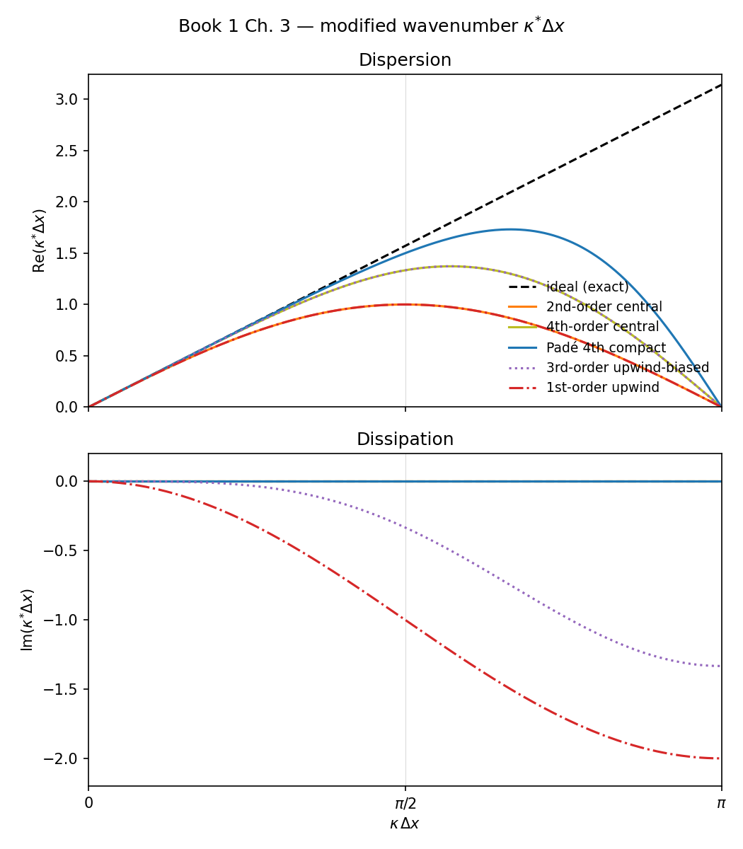
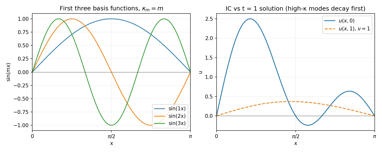
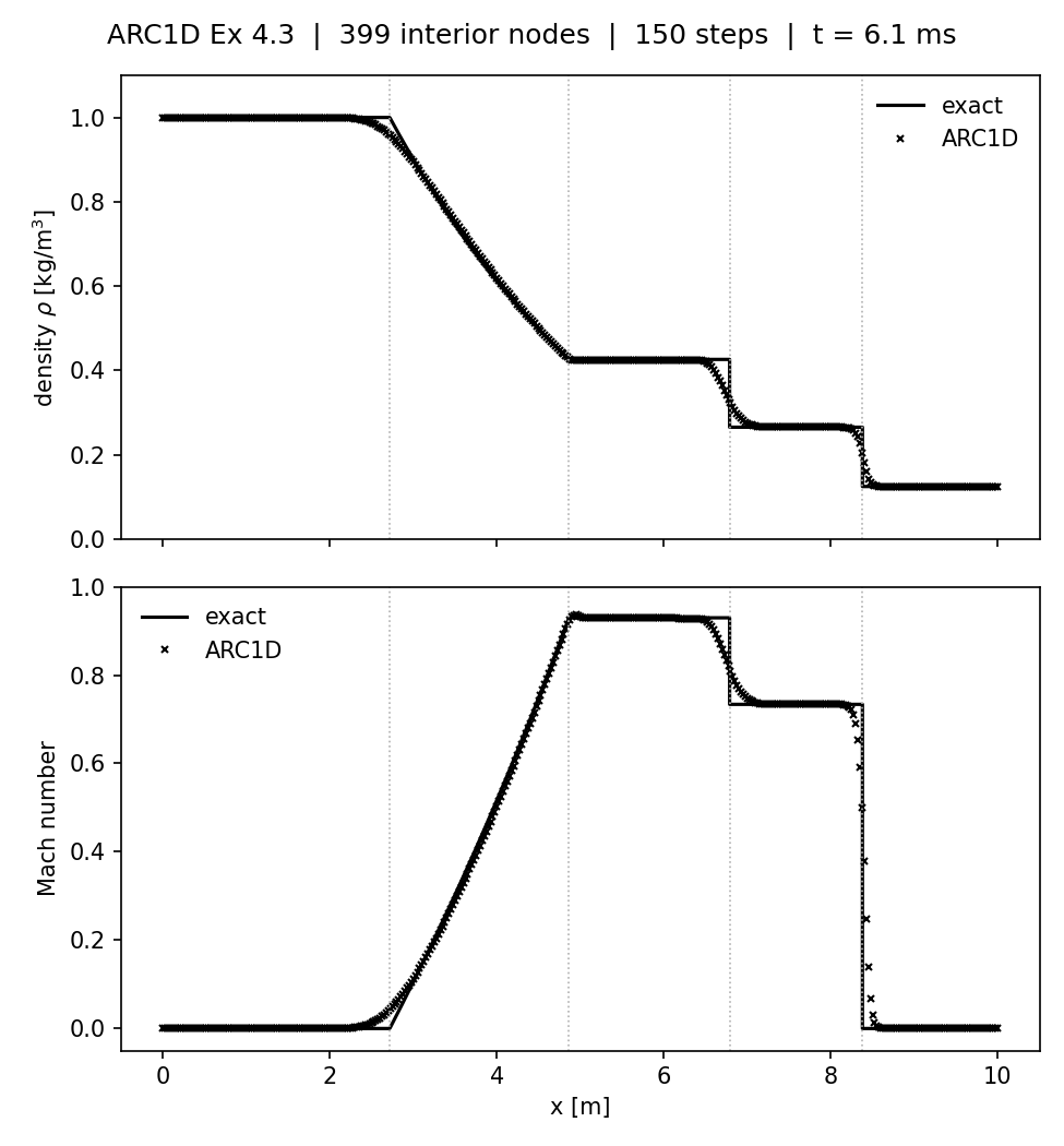
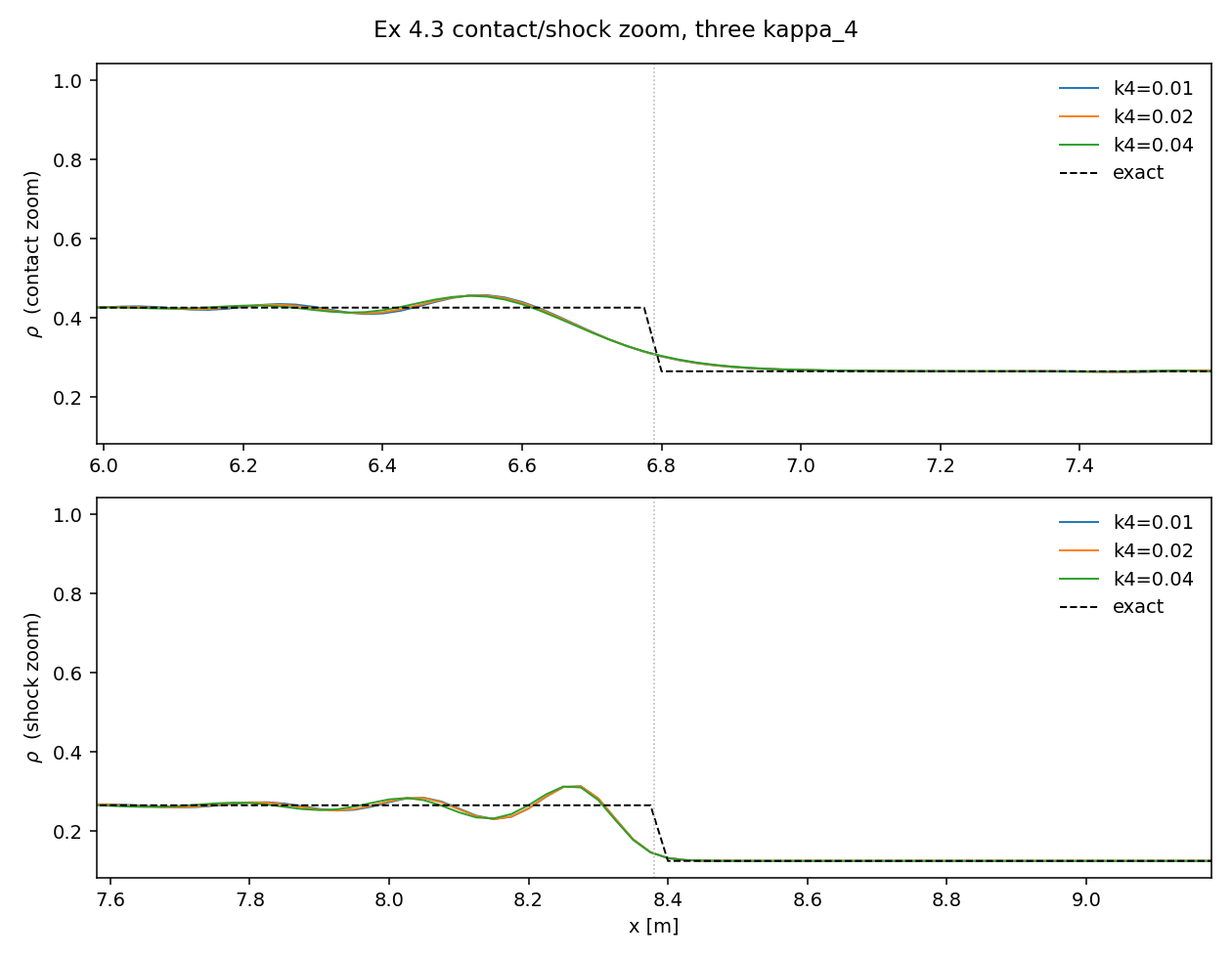
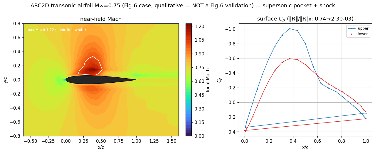
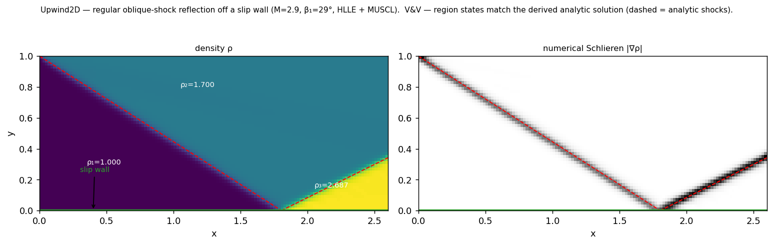
These are the other results the same codebase produces, each rendered by the script that owns it, and each one is a different chapter of the two books the project works through.
What this does not establish
- One case, one grid family, one final time. Verification against an exact solution, not validation against an experiment.
- The two solvers differ in more than the flux: JST runs 150 fixed implicit steps at Courant 1, Roe runs adaptive SSP-RK2 at CFL 0.8. The comparison is of two complete schemes, not of two flux functions in isolation.
- Grid convergence of the transition width itself is not shown. These are single-grid results, so the 1.6 is a ratio at this Δx and not an asymptotic statement.
- The mechanism given above (a pressure sensor that cannot see a contact) is the standard explanation and is consistent with the measurement. It is not itself measured here; no sensor field is dumped from either run.
Where the timestep stops working, and what buys a bigger one
Drive it · linear model problemChapter 01 runs 150 implicit steps at Courant 1 and never says what happens at Courant 2. This is that question with a control on it: one pulse, a periodic box, and a stability limit that moves when you pay for it.
Set the two numbers, then run. The pulse has to go four times round the box and still be a pulse.
What this is. Linear scalar convection on a periodic box, second-order central in space, marched by the five-stage scheme FLOMG ships, with implicit residual smoothing. The curve is exact for that. It is not the Euler solver: no nonlinearity, no shock, no characteristic boundaries, no fourth-difference dissipation. The squares are what the nonlinear solver measured, and they are a bracket rather than a number.
Narration
01 What the control marches
Linear scalar convection on a periodic box, 200 cells, second-order central in space, and the Jameson five-stage Runge-Kutta the solver ships, with stage coefficients (1/4, 1/6, 3/8, 1/2, 1). The task is to carry the pulse four times round the box and get it back still a pulse, in as few steps as possible. A bigger Courant number is fewer steps, so the whole game is how big a one you can get away with.
02 Where the cliff is, exactly
Implicit residual smoothing replaces each stage's residual R by the R̄ that solves R̄ − βδ²R̄ = R. Per mode that divides the amplification argument by 1 + 4βsin²(θ/2), so the largest argument the march ever sees is Cn/√(1+4β), and the five-stage polynomial is stable along the imaginary axis out to |z| = 4. The cliff is therefore closed form:
Cnmax(β) = 4√(1 + 4β)
A square root, not a straight line. Three times the timestep costs β = 2, and the slider runs out before it. Push it and the diminishing return is the thing you feel first.
03 Why the squares are not the curve
The curve is a model problem and the squares are the solver. They are different objects. The squares are the measured integer bracket on the real nonlinear march at J = 105 over a 400-step window, filled on the last stable value and hollow on the first unstable one, and the same bracket came back on the subsonic and the transonic exercise. Where the curve falls inside a bracket the two are consistent, which is all that can be said. At β = 0 the curve sits exactly on the first unstable integer, and past the last measured β there are no squares at all.
04 Why a doomed run looks healthy
Over the cliff the worst mode multiplies by max|σ| every step, starting from whatever seeds it. Here that is a stated broadband perturbation of 1e−9, standing in for the round-off a real march starts with. Two per cent over the cliff is a growth of about 1.35 a step, which needs roughly seventy steps to climb from that seed to anything a plot can show, and until then the pulse is clean. The nonlinear solver's own runs say the same thing: at β = 0.2 an unstable run goes non-finite in eight steps, and at β = 1.0 the same verdict takes 101 steps of the 400-step window on the subsonic exercise and 91 on the transonic one. Nothing in the upper panel knows. The dashed trace, the hatching and the map do.
How many sweeps it takes to get the error off the grid
Drive it · linear model problemA second control, on the other half of the cost of a steady solution. Not how big a step you may take, but how many sweeps it takes to get the error off the grid, and why the answer is not to sweep harder.
The error on the grid is one low mode and one high mode. Get the residual to one part in a million before the allowance runs out.
What this is. The linear 1-D Poisson model problem, −u″ = f on the unit interval with Dirichlet ends and second-order central differences. It is the output of the relaxation chapter and the input of the multigrid chapter. It is not a statement about how the nonlinear Euler solver converges, and the work-unit numbers here are this problem's, not that solver's.
Narration
01 The grid is the error
Take f = 0, so the exact answer is zero and whatever is left on the grid is the error. It starts as two modes: the lowest one the grid can hold, and a high one drawn fresh out of the band ξ ∈ [π/2, π] at every restart. Drawn rather than fixed, because a single fixed high mode has a weight that annihilates it exactly, and that weight is not the answer. The band is what the smoothing factor is defined over, so the band is what you have to beat.
02 One eigenvalue per mode
Weighted Jacobi has a single number per mode: μk(ω) = 1 − ω(1 − cosξ), with ξ = κΔx. The smoothing factor is the worst of those over the high band, and it is smallest at ω = 2/3, where it is 1/3. Plain Jacobi, ω = 1, is the worst setting on the slider: at ξ = π it has |μ| = 1 and does not touch the Nyquist mode at all. The control opens there. Press smooth and watch how little happens.
03 What the coarse grid is for
One smooth is one sweep of the fine grid and costs one work unit. One coarsen is a two-grid cycle: two sweeps, the residual, full-weighting restriction to the half grid, an exact solve there, linear prolongation back, the correction, two more sweeps. The repository prices that at about 4.25 work units, and that number is the whole comparison, because a method that is four times the work per step has to be four times better to be worth anything. The readout says what each mode would cost the smoother on its own. At ω = 2/3 the high mode is gone in at most thirteen sweeps whatever the restart drew, and no weight on this slider takes the lowest mode under nine thousand. That gap is the entire reason multigrid exists.
04 What it does not say
This is one linear model problem with a known spectrum, which is why every number on it can be computed rather than measured. FLOMG's multigrid tables are the measured article and they are a different reading, including two failures worth as much as the successes: a five-level hierarchy at J = 105 that is invalid because the grid nesting breaks, and a V-cycle on the transonic case that never reaches 1e−12 in 300 cycles.