Independent · ongoing

A new case swaps a mesh and inherits every convergence, discretisation and post-processing decision unchanged.

An OpenFOAM external-aerodynamics pipeline built around the Ahmed body, with the discipline in the templates rather than in someone's memory, and one study.

Solver: simpleFoam · steady SIMPLE · k-ω SST
Baseline: AHMED-25_FG_M22, 7 922 294 cells, 3 600 iterations
Evidence here: Field data, sampled 2026-09-03
Register: Benchmark and error characterisation

Pressure coefficient on the centreline plane of the baseline case AHMED-25_FG_M22: 7 922 294 cells, 3 600 iterations of steady SIMPLE. Blue is suction down to C_p = −1.25, warm is above ambient to +1.05, and the pale centre is zero. Sampled from the solver's own written field.

A single external-aerodynamics case has enough moving parts (geometry, mesh, boundary conditions, solver, closure, post-processing) that untracked variation drifts the answer faster than the physics does. The pipeline's whole purpose is that the parts which decide what is measured are fixed in the template, and only the part under study moves.

Across the 33 cases of the mesh-independence sweep the dictionary that defines the force measurement has exactly one version, so every case measures drag the same way. The six runs that settled were not otherwise identical: they also vary the inlet turbulence and, on one run, the momentum scheme, so the spread between them is not attributable to the mesh. What follows is that comparison, plus the flow field the baseline case produced: sampled from the solver's own written fields.

It also found something. Holding the measurement fixed is what makes a discrepancy visible instead of absorbable, and the discrepancy this one surfaced is in the geometry it was run on. Chapter 04.

The baseline case, M22

U_∞: 30 m/s
ν: 1.5 × 10⁻⁵ m²/s
Re_L: 2.09 × 10⁶
cells: 7 922 294
iterations: 3 600
ground: fixed, no-slip
wall: functions, ȳ⁺ 74.8
C_d: 0.2281

The flow the baseline case produced

The evidence

One object. Every state below is the same converged solution read a different way: the symmetry plane in two quantities, then a series of cross-planes stepping from the slant leading edge into the near wake. Every frame is sampled from the solver's own field files.

Narration

01 The symmetry plane

Streamwise velocity through the centreline, as a fraction of the 30 m/s freestream. Everything below zero is reversed flow: a closed recirculation sitting immediately behind the slanted rear, and a second one under the body. The same plane in pressure coefficient. The stagnation point reaches Cp = 1.00, which is the arithmetic the normalisation has to satisfy and the first check that the sampling is sound.

02 Across the slant

Streamwise vorticity at the slant leading edge. The flow has just been asked to turn downward and the side edges are already shedding. Half way down the slant, a counter-rotating pair is clearly formed: one sign each side of the centreline. Near the base, the pair has moved inboard and strengthened.

03 Into the wake

At the base, the longitudinal pair sits above the blunt-base recirculation rather than in it. Sixty millimetres downstream the peak magnitude has fallen and the pair has spread. Three hundred millimetres downstream it is what it was at the base, and diffuse. The structures are present and they spread rather than disappear, which is what a steady RANS closure on this mesh is able to say about them; the next chapter measures it.

The field frames are sampled from the solver's own field files. Without scripting: the baseline case AHMED-25_FG_M22 converged to C_d = 0.2281 at 7.92 M cells and 3 600 iterations, with a closed recirculation behind the slant and a counter-rotating longitudinal vortex pair whose circulation at 300 mm downstream matches its base value within 1 %, with a dip between, while its peak vorticity falls by a factor of 3.8.

The field, as the solver rendered it

The panels above are rebuilt from the extracted arrays. These two are the renders themselves, and they carry the one thing an extracted slice cannot: what the structure looks like in three dimensions.

A velocity field on the symmetry plane of an Ahmed body: fast red flow over and around a blue low-speed body, with a long blue wake trailing behind the slanted rear and a thin shear layer between them. — 2024 Velocity on the symmetry plane. The blue region behind the slant is the separated wake, and its length is what the drag coefficient is mostly reporting.

Q-criterion isosurfaces behind an Ahmed body, rendered in green: a pair of long counter-rotating trailing vortices springing from the slant edges and breaking into smaller structures downstream. — 2024 Q-criterion isosurfaces. The two long tubes are the C-pillar vortices that form at the edges of the slant, and they are the reason the twenty-five degree Ahmed body is a benchmark at all: change the slant angle a few degrees and they stop forming.

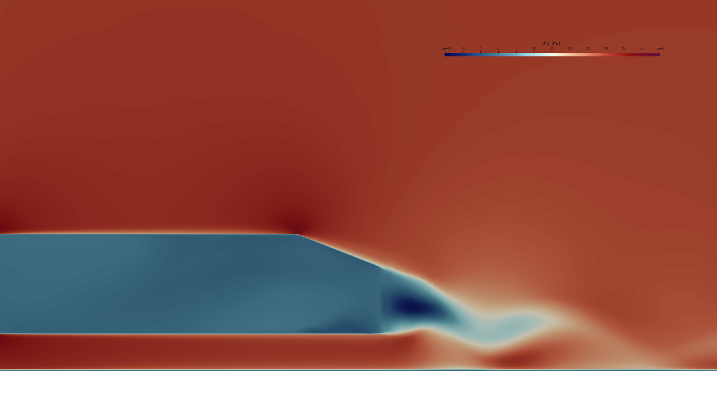
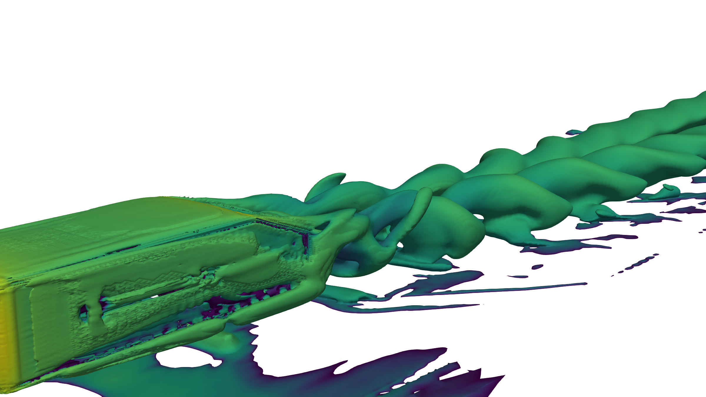
The wake does not fade. It spreads.

Circulation

A slanted-back bluff body at this angle does something specific: the flow spilling off the two side edges of the slant rolls into a pair of counter-rotating longitudinal vortices, and those vortices hold the flow attached over a surface that ought to have separated. Looking at the planes tells you the pair gets fainter downstream. Integrating them tells you that at 300 mm its circulation is back to the base value, with a dip between.

Circulation is the area integral of vorticity over one vortex, and it is the quantity that is conserved when a vortex diffuses. Both numbers below are computed here from the committed cross-plane arrays: the same-sign vorticity summed over the half-plane one vortex occupies, with nothing fitted.

The same integration gives the core's position: the intensity-weighted centroid of one vortex, plotted from behind. Circles are the eight stations, from the slant leading edge to 300 mm downstream. The rectangle is the body's own cross-section at the base.

Those are the planes the numbers above were measured on. Each panel is scaled to its own peak, because a shared scale would flatten the last three into grey, and the peak is printed instead so the comparison a shared scale would have made is still available.

What the sweep does, and does not, show

The limit of the claim

Six runs reached a settled tail and are plotted. Two did not settle and are not plotted:

Read the settled six left to right and C_d does not settle with them.

That is the result of this study. Grid independence needs a refinement ratio around 1.3 in cell size across at least three levels: roughly 2.2× in cell count per level. The six settled runs span 7.88 M to 10.77 M, a factor of 1.37 in count and about 1.11 in size. It is not wide enough to demonstrate independence, and it does not. Nor is it one mesh family run identically: M22 and M24 share a mesh to the cell and differ in inlet turbulence, M29 has a third inlet setting, and M34 uses a different momentum scheme from the other five. The spread is not attributable to the mesh. What the sweep does establish is that every case measured drag through the same force dictionary.

What the run was checked on

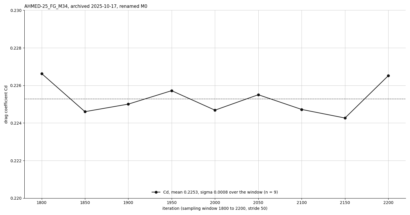
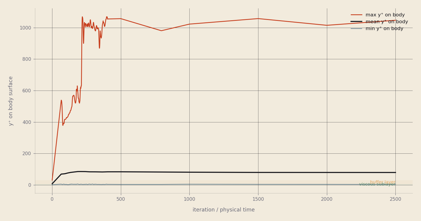
A force coefficient means nothing without the two figures beside it: how far it had settled, and whether the mesh was resolving the wall at all. Both are from the archived run AHMED-25_FG_M34 (renamed M0, 8.4 M cells), which is neither the M22 baseline above nor the 9.75 M-cell M34 in the sweep.

Drag coefficient of the archived run AHMED-25_FG_M34 at nine samples between iteration 1800 and 2200: points within 0.0008 of a dashed mean line at 0.2253. — 2024 Drag coefficient of the archived run AHMED-25_FG_M34 (renamed M0) at each sample of the 1800 to 2200 window: mean 0.2253, standard deviation 0.0008 over nine samples. A converged number is one that stops depending on where you start averaging.

Wall y-plus against iteration: a maximum curve that spikes early and settles near a constant, with mean and minimum curves flat and much lower. — 2024 Wall y-plus over the archived run AHMED-25_FG_M34 (renamed M0): body mean about 82 over the last hundred samples. This is the figure that says whether the turbulence model is being used inside its own assumptions: the wall functions need the first cell centre in a particular range, and if it is not, the drag number is answering a different question than the one asked.

The geometry the sweep was run on

What the discipline caught

Every coefficient quoted above is normalised by a reference area, and every comparison to published work assumes a shape. Both were checked against the triangulation the solver meshed: constant/triSurface/body.stl, byte-identical in all four converged cases.

Length and width are the Ahmed body's. Height, ground clearance and slant angle are not, and they are wrong together: scaling the standard body by 0.852 in z alone gives a height of 0.2454 m and turns a 25° slant into atan(0.852·tan 25°) = 21.67°, which is what the triangulation measures to three decimals.

The reference area declared to the force calculation is 0.112032 m²: exactly 0.389 × 0.288, the standard body's frontal area. The frontal area of the triangulation, computed exactly from the mesh, is 0.095459 m². The declared reference is 1.1736× the geometry's own.

What that does and does not affect. The sweep compares cases that all share this geometry and this reference, so the mesh comparison above is unaffected: a constant factor divides out of it. What it forbids is the comparison this case's name invites: these coefficients are not on the same footing as published 25° Ahmed-body data, and none is set beside them here. The cause of the scaling is not established here; only the measurement is.

Measured from the meshed triangulation, against the standard body
quantity	this STL	Ahmed 1984	ratio

Rows that disagree are marked. Standard values as tabulated in the ERCOFTAC AC1-05 case description of Ahmed, Ramm & Faltin (1984), SAE 840300.

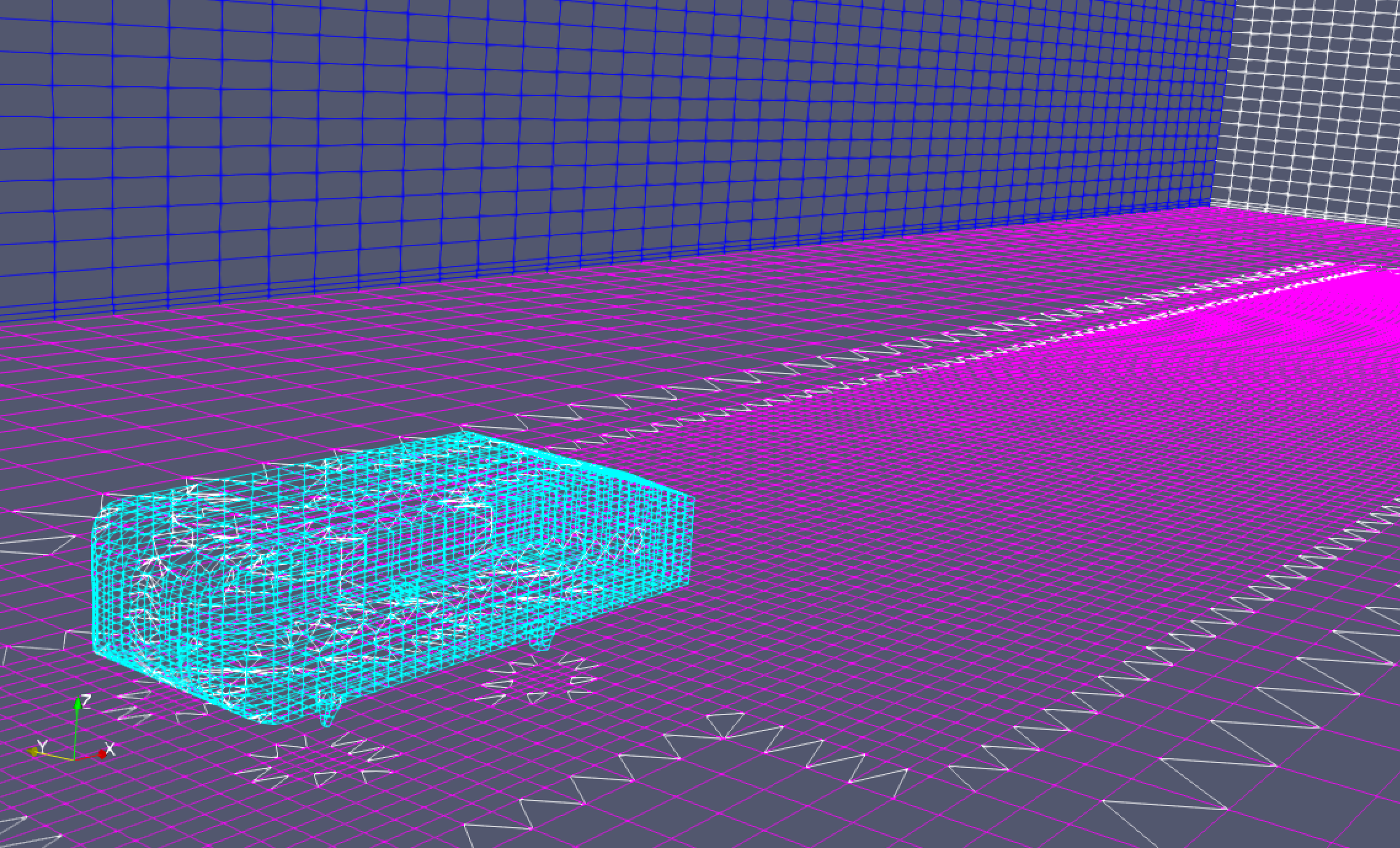
A cut through the volume mesh around the Ahmed body: a cyan refined cell cluster hugging the body, a magenta and blue graded background mesh, and a structured grid on the ground plane and far field. — 2024 The mesh the sweep ran on, cut open. The dense cyan region is the refinement that has to be there for the wake to exist at all; everything outside it is graded away as fast as the solver will tolerate, because cells spent far from the body are cells not spent on the separation.

The strongest thing the case can say is not a drag coefficient. It is that a pipeline built to hold the measurement fixed did exactly that, and the first thing it caught was an inconsistency in its own baseline case: a body scaled in z and a reference area that was never rescaled with it. A study with the force dictionary edited per case would have absorbed that as scatter and nobody would have looked. Here it is a 1.1736× factor with a number on either side of it.

The repair belongs in the case: re-cut the geometry or declare the geometry's own frontal area, then re-run. Until that happens the mesh comparison stands, the flow field stands, and the coefficient stays off the literature axis.

What this does not establish

Not a validated drag prediction. The geometry is a 21.67° slant with a 0.2454 m height, and the coefficients are normalised by the standard body's frontal area rather than its own. No comparison to published Ahmed-body coefficients is made on this page; the y⁺ note makes a drag-level one, and with this slant and reference area it can only be drag-level.
Not grid independence. Six settled runs spanning 7.88 to 10.77 M cells is a refinement ratio of about 1.11 in cell size, and they differ in inlet turbulence and, on one run, the momentum scheme. C_d varies by across them with no monotone trend.
Every case in the repository runs simpleFoam: steady SIMPLE, with endTime as an iteration count. Nothing here is time-resolved, so the vortex structures are a steady RANS closure's time-averaged picture of them and carry no unsteady content at all. The two cases named _SAS and _DES also declare simpleFoam and produced no result.
Wall treatment is the wall-function regime. Measured body y⁺ on the M22 baseline averages 74.8, inside the 30–300 band, but reaches 840 at its maximum, which is outside it. Not resolved to the wall anywhere.
Sampling gaps: a cutting plane returns values where it crosses cells, so 27 % of the rendered grid had no sample and takes the value of the nearest one. For a finite-volume field, which is piecewise constant over a cell, that is what the solver's data says holds there, but it is a rendering choice.

What I would do differently

Earlier benchmarking would have saved time. My first Ahmed body run had enough drag error that I spent longer than I should have chasing mesh sensitivity, when the shortcut, binding the geometry's reference dimensions and running a known-good reference case alongside every new one, belonged at the top of the template.

Next is the DrivAer geometry, which is a real car shape rather than a bluff body with a slant, and it is where a template that only ever worked on the Ahmed body would stop being useful.

Open thread

Ahmed body: a y⁺ pass on the baseline grid

All open threads →